Contents
IntroductionNearest-neighbour interpolation
PDE-based interpolation
Laplace PDE
Biharmonic PDE
Application to TSP
References
Introduction
In this post, I'd like to present a visualization technique complimentary to nonlinear dimensionality reduction methods. Interpreting their results can be difficult because unlike the linear methods such as PCA, there are no axes corresponding to the data features. It'd be nice to have a kind of map indicating how the original features change across the nonlinear projection. Such a map can be built via interpolation in the projection space. The task is complicated by the fact that we're dealing with a scattered data not lying on a uniform grid and must choose a suitable interpolation method.
Nearest-neighbour interpolation
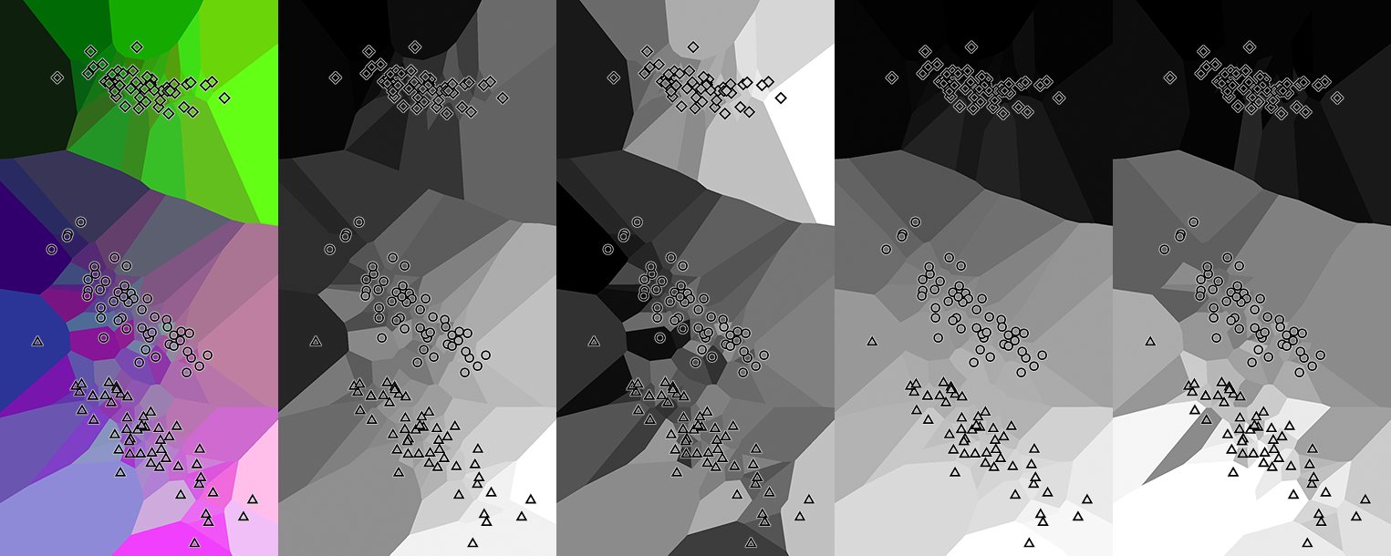
Colouring each pixel according to some feature of the nearest projected point (nearest neighbour interpolation) is the simplest method. Although it gives the general idea of the feature behaviour, the resulting feature maps are not smooth and contain huge nasty looking Voronoi cells in case of uneven point distribution. I shall use the MDS of the classic Iris dataset for illustrations. The features have been preprocessed using the unit mean normalization and collinear inflation correction (see InvMem 25 for details). The image depicts four individual feature maps and a false-color composite one whose RGB channels correspond to the first three features. Diamonds, circles and triangles correspond to setosa, versicolor and virginica species respectively.
PDE-based interpolation
Fortunately, there is another class of interpolation methods well suited for scattered data: partial differential equation (PDE)-based interpolation. The idea is to find a solution of a PDE satisfying the condition of assuming specific values at specific points. I have implemented two PDEs: Laplace equation ∆f = 0 and the biharmonic equation ∆2f = 0, where ∆ = δ2f / δx2 + δ2f / δy2 is the Laplace operator. Since we are solving the PDEs on the pixel grid, we'll use a discrete version of the ∆ or ∆2 operator called a stencil or a kernel K. From the condition ∑fx + i, y + j Ki, j = 0 we can obtain the Jacobi relaxation iteration: fx, y, t + 1 = ∑fx + i, y + j, t Ki, j / K0, 0, i2 + j2 > 0, or simply ft + 1 = ft − ft ∗ K / K0, 0, where ∗ stands for convolution. The PDE can be solved by repeating the iteration while leaving the prespecified points unchanged.
However, to ensure stability a slightly different underrelaxed iteration should be employed: ft + 1 = ft − ft ∗ K / C, C > K0, 0. The iteration applied to a checkerboard pattern should not lead to unbounded oscillations, so |C| ≥ |∑ Ki, j|, (i + j) mod 2 = 0. Another notable issue is impractically slow convergence for large image sizes. Fortunately, the solution process can be accelerated with the aid of a multiscale approach: first, solve the PDE at a low resolution, then upscale the solution and continue in this manner until the desired resolution is obtained.
Laplace PDE
Two possible Laplace operator discretizations are
| L5 = |
| 1 | ||
| 1 | -4 | 1 |
| 1 |
| , L9 = |
| 1 | 4 | 1 |
| 4 | -20 | 4 |
| 1 | 4 | 1 |
| / 6, |
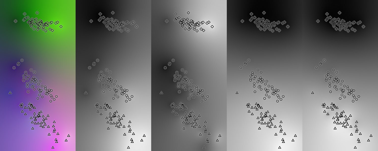
the latter being more accurate. From the physical perspective, the solution to the Laplace equation describes a stationary temperature distribution. Although the resulting images are smooth, they look hazy:
Biharmonic PDE
Discrete bi-Laplace operator can be obtained by convolving a Laplace operator with itself:
| BiL13 = |
| 1 | ||||
| 2 | -8 | 2 | ||
| 1 | -8 | 20 | -8 | 1 |
| 2 | -8 | 2 | ||
| 1 |
| , BiL25 = |
| 1 | 8 | 18 | 8 | 1 |
| 8 | -8 | -144 | -8 | 8 |
| 18 | -144 | 468 | -144 | 18 |
| 8 | -8 | -144 | -8 | 8 |
| 1 | 8 | 18 | 8 | 1 |
| / 36 |
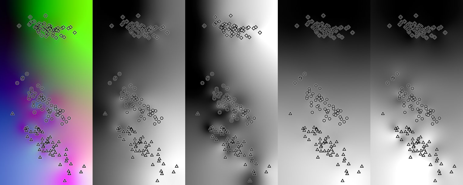
A solution of the biharmonic equation also has a physical interpretation: it describes a thin elastic plate having the minimal bending energy. The resulting images look much cleaner in comparison to the Laplace PDE:
Application to TSP
Finally, I'd like to present an application I find to be particularly interesting. Let's consider solutions to the travelling salesman problem (TSP) - that is, closed tours visiting all of the specified locations on the Euclidean plane just once. Moreover, let's only consider 2-opt locally optimal solutions - that is, tours that cannot be improved by cutting two edges and replacing them with two different ones. The distance between two solutions can be defined as the number of mismatched tour edges. For this example, I chose the PCB442 instance from TSPLib. Here are the normalized tour length MDS maps (the color scheme is Hesperia) with the global optimum marked:
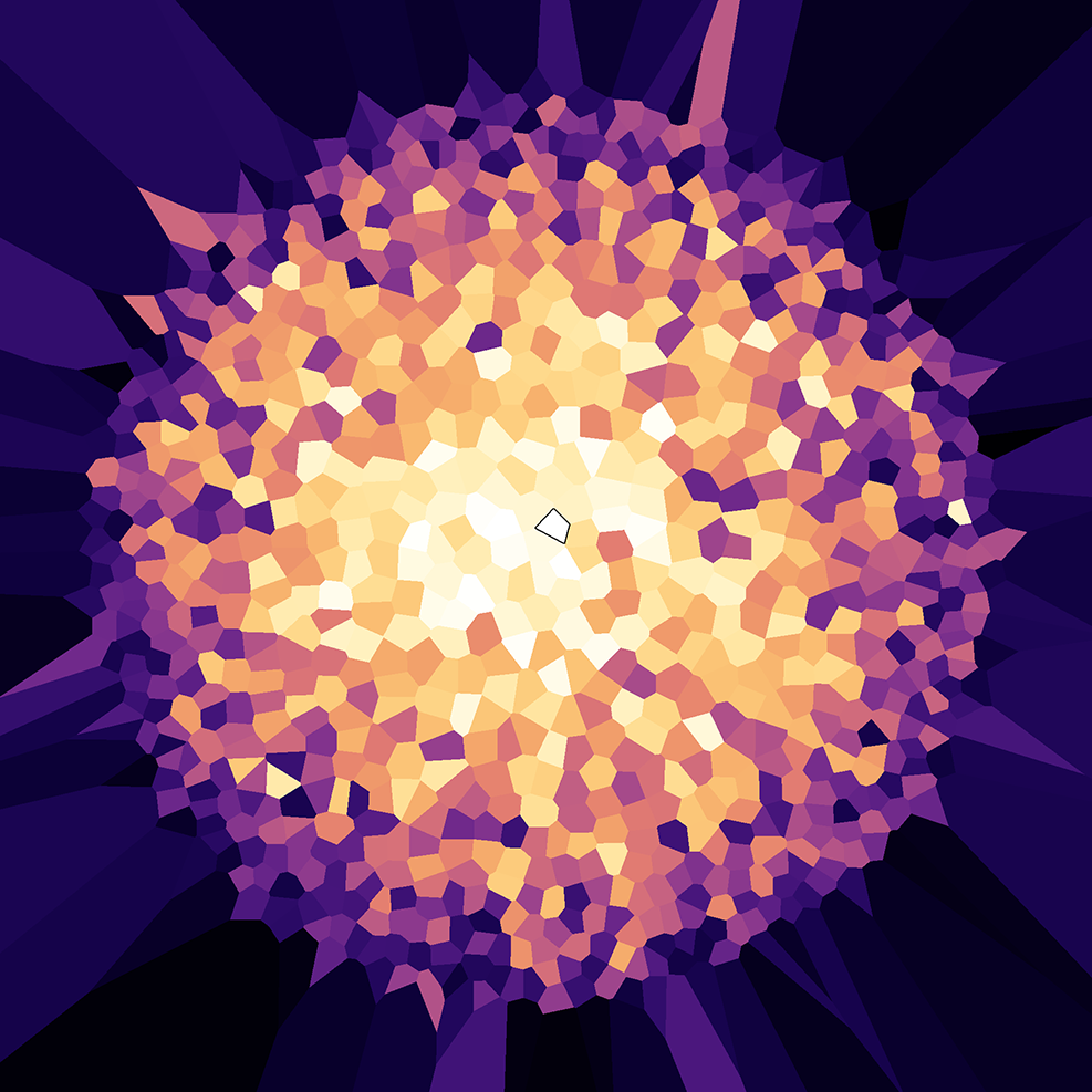
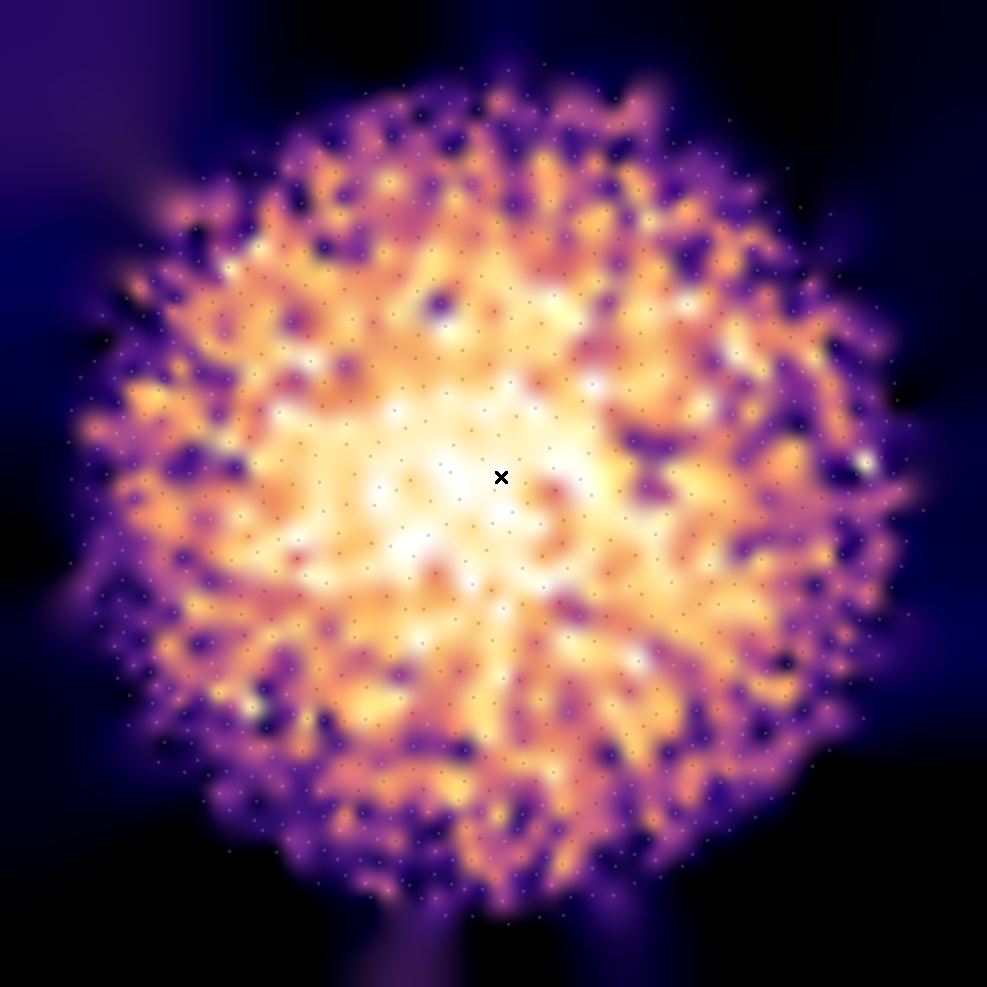
The images reveal an important feature: shorter tours lie closer to the center, and that is where the global optimum is located. Fitness-distance correlation is, in fact, a well-known phenomenon reported in [1]. But I find this kind of search space map to be more illuminating than the correlation coefficient alone. It is pretty neat how the MDS feature map gives us a glimpse into a space combinatorial in nature.
References
- Boese K D. Cost Versus Distance In the Travelling Salesman Problem.