InvMem is a collection of short notes on mathematics and programming.
Contents
N1 / Kepler-style coincidences / #Math / 2014.09.23
Take a Kepler triangle - a right triangle with sides 1, √φ, φ. Then the length of its circumscribed circle nearly matches the perimeter of a square with a side equal to its middle edge. This yields an approximation τ ≈ 8 / √φ. Here are some coincidences having a similar form:
| Constant | Approximation | Relative Error |
|---|---|---|
| τ | 12 / 5 φ2 | 1 / 65270 |
| τ | 9 / 2 3√e | 1 / 2144 |
| τ | (11 / 7)3 φ | 1 / 1409 |
| τ | 8 / √φ | 1 / 1043 |
| e | 3√10 / 7 S | 1 / 3770 |
| e | 7 / 4 √S | 1 / 3305 |
| e | 5 / Ln τ | 1 / 1210 |
| e | 9 / 8 S | 1 / 1186 |
| γ | 1 / √3 | 1 / 4289 |
| P | √8 / 11 S | 1 / 3841 |
| P | 9 / 11 φ | 1 / 1519 |
| Notation: | |
| τ | Circle constant |
| e | Base of the natural logarithm |
| φ | Golden ratio |
| S | Silver ratio |
| P | Plastic number |
| γ | Euler-Mascheroni constant |
N2 / Note on means / #Math / 2015.02.10
Consider a family of means of two numbers a, b:
M(a, b, p) = ∫abxp + 1 dx / ∫abxp dx
In other words, M(a, b, p) is the mean of a distribution with density ∝ xp in the interval [a, b]. Many well known means belong to this family:
| p | Expression | Name |
|---|---|---|
| 1 | (2 / 3) (a + b - a b / (a + b)) | ??? |
| 0 | (a + b) / 2 | Arithmetic |
| -1/2 | (a + √a b + b) / 3 | Heronian |
| -1 | (b - a) / (Ln b - Ln a) | Logarithmic |
| -3/2 | √a b | Geometric |
| -2 | a b (Ln b - Ln a) / (b - a) | ??? |
| -3 | 2 a b / (a + b) | Harmonic |
N3 / Generalized Motzkin numbers / #Math / 2015.02.16
Number of strings of length N consisting of symbols from the alphabet of size b and correctly placed brackets is
| ⸤N / 2⸥ | |
| ∑ | (N | 2 i) bN - 2 i Ci , |
| i = 0 |
where (N | 2 i) is a binomial coefficient and Ci is the ith Catalan number. This result is easy to interpret: Ci is the number of possible configurations of 2 i brackets, (N | 2 i) is the number of ways to place a bracket configuration among the N symbols, and bN - 2 i is the number of possible configurations of the non-bracket symbols.
| b | OEIS | First terms starting with N = 0 | |
|---|---|---|---|
| 0 | A126120 | 1, 0, 2, 0, 5, 0, 14, 0, 42, ... | Catalan numbers interleaved with 0s |
| 1 | A001006 | 1, 1, 2, 4, 9, 21, 51, 127, 323, ... | Motzkin numbers |
| 2 | A000108 | 1, 2, 5, 14, 42, 132, 429, 1430, 4862, ... | Catalan numbers |
| 3 | A002212 | 1, 3, 10, 36, 137, 543, 2219, 9285, 39587, ... | |
| 4 | A005572 | 1, 4, 17, 76, 354, 1704, 8421, 42508, 218318, ... | |
| 5 | A182401 | 1, 5, 26, 140, 777, 4425, 25755, 152675, 919139, ... | |
| 6 | A025230 | 1, 6, 37, 234, 1514, 9996, 67181, 458562, 3172478, ... |
N4 / Scale derivative / #Math / 2015.02.28
Derivative of f(x) is defined as the limit (f(x + h) - f(x)) / h, h → 0. By replacing the shift f + h with scaling x / s, we obtain the scale derivative: g(x) = Limit (f(x / s) - f(x)) / Ln s, s → 1. In the logarithmic x scale, scaling is equivalent to shifting and scale derivative to the normal derivative: t = Ln x; q(t) = f(x); g(x) = Limit (q(t - Ln s) - q(t)) / Ln s, s → 1 = -dq(t) / dt = -df(x) / d Ln x = -x f'(x). It is assumed that x > 0. For x < 0, same results apply in a mirrored form.
g(x) to f(x) is what a gnomon is to the figurate numbers. Infinitesimally larger version of f(x) is obtained by adding g(x) to it: f(x / s) ≈ f(x) + g(x) Ln s. We can continuously "grow" f(x) in size by adding infinitesimal amounts of scaled g(x). Under the condition f(∞) = 0, the original function can be reconstructed as a superposition of g(x) with exponentially increasing scales: f(x) = ∫-∞0 g(x / ez) dz, z = Ln s. This is easily proven by using the identity g(x) = -dq(t) / dt. If the upper integration limit is different, f(x) is obtained at the corresponding scale.
Alternatively, f(x) can be seen as being reconstructed from area-normalized g(x) at scales from 0 to 1: f(x) = ∫01g(x / s) / s ds. We can "grow" the distribution with PDF equivalent to f(x) by sampling from PDF ∝ g(x / s) starting with s = 0 and increasing it linearly. At any time, distribution of all the values generated so far will match f(x) up to scaling. This trick will only work if f(x) is non-increasing. Otherwise, g(x) will contain negative values and cannot be a proper PDF.
N5 / Generating generalized Gaussian, Cauchy and related random variables / #Math #Algorithms/ 2015.03.31
Consider a generalized Gaussian (PDF ∝ e-|x|p) and generalized Cauchy (PDF ∝ 1 / (1 + |x|p)) random variables. An easier to sample bounding functions are required to apply the rejection sampling technique. It is easy to verify that both distributions are log-log convex upwards. Therefore they can be bounded by tangent lines in the log-log scale - that is, by power functions. Piecewise power law PDFs are easily handled by inversion sampling of their pieces with corresponding probabilities. It suffices to sample the x > 0 half of the distribution and symmetrize it by multiplying the results by ±1 at random.
Let's bound f(x) ∝ PDF with h(x) consisting of two segments: h(x) = 1 if x < x1, A x-q otherwise. The segments match at x1, so x1 = A1 / q. Area below h(x) is S = A1 / q (1 + 1 / (q - 1)). The efficiency (acceptance rate) is ∫0+∞ f(x) dx / S. Let's denote the point where h(x) touches f(x) as xe. Then A = f(xe) xeq and q is the log-log slope of f(x) at xe. Expressing A through q and solving dS / dq = 0 yields the optimal q. This process leads to a transcendental equation for the generalized Cauchy density: q / (1 - q) = Ln(1 - q / p). A slightly less efficient function that avoids the problem is obtained by assuming q = p (tangent at +∞).
| Name | f(x) | q | A | Efficiency | Min efficiency |
|---|---|---|---|---|---|
| Generalized Gaussian | e-|x|p | p + 1 | ((q / p) / e)q / p | (p-1! e1 / p) / (1 + 1 / p)1 + 1 / p | 0 at p → 0 |
| Generalized Cauchy | 1 / (1 + |x|p) | p | 1 | τ (p - 1) / (2 p2 Sin(τ / (2 p))) | τ / 8 at p = 2 |
Scale derivatives of the examined functions can be enclosed with three segments: xp if x < x1, M if x < x2, A x-q otherwise, where M = Max f(x). Scale derivative of Cauchy density can be effectively sampled by assuming q = p. In the Gaussian case, optimal q is a solution to the transcendental equation (1 / p + 1 / (1 - q)) q = Ln(1 + q / p). Approximate solution obtained with the aid of Newton's method is listed in the table below.
| f(x) | M | q | A | Min efficiency |
|---|---|---|---|---|
| xp e-|x|p | 1 / e | Max((15 / 7) p + 13 / 19, 1 + p) | ((1 + q / p) / e)1 + q / p | 0 at p → 0 |
| xp / (1 + |x|p)2 | 1 / 4 | p | 1 | 2 / (1 + Ln 4) at p → +∞ |
N6 / Triplane hexagonal coordinates / #Math #Programming #Board_Games / 2015.04.06
Consider a hexagonal-shaped region of a hexagonal grid. A coordinate system can be formed by three semi-axes 120° apart starting from the center of the region.
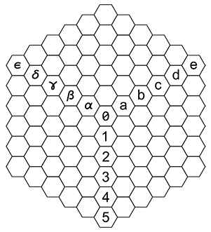
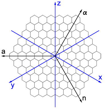
The system is well suited for board games. Most hexagons are encoded with combinations of two symbols. Axis hexagons are encoded with one symbol. Compared to existing hexagonal chess variants, the system has a pleasant symmetry. Each symbol except 0 appears in equal number of hexes. Hexagonal array can be efficiently stored as three rectangular arrays overlapping at the axes. Conversion to the cubic (3D) coordinates is straightforward: triplane coordinates (n, a, α) are equal to the absolute values of the coordinates of 3D axes (x, y, z) lying in the corresponding sector: (n, a) = (-z, y), (a, α) = (-x, z), (α, n) = (-y, x).
N7 / Short brainfuck programs / #Programming / 2015.04.22
Following programs were generated with Ascension framework. Memory cells are assumed to be integers [0 .. 255], wrapping around.Text output:
| Program | Length | Output |
|---|---|---|
| +>-[>>+>+[++>-<<]-<+<+]>---.<<<<++.<<----..+++.>------.<<+.>.+++.------.>>-.<+. | 79 | Hello World! |
| +[-[<<[+[--->]-[<<<]]]>>>-]>-.---.>..>.<<<<-.<+.>>>>>.>.<<.<-.<<+. | 66 | hello world! |
For comparison, shortest human-coded "Hello World!" program is 89 instructions long:
++++++++++[>>->++>+++>+++>----->+[++++++++<]<-]>>++.>+.>--..>+.>++.>---.<<.+++.<.<-.>>>+.
Calculating sequences in memory:
| Program | Length | Output |
|---|---|---|
| -[+>+>--[<]>>] | 14 | Powers of 2 |
| +[>>-->+[<]<+] | 14 | Powers of 2 |
| >-[[<+>>>-<-<+]>] | 17 | Fibonacci sequence |
| >-[[>-->+<<<+>+]>--] | 20 | Squares |
N8 / Lattice distance distortion / #Math / 2015.05.17
Take a regular lattice with each point connected to a few neighbouring points, thereby forming a graph. Let's only consider physically meaningful neighbour sets: a line connecting a lattice point to any of its neighbours should not intersect other Voronoi cells in more than one point. This requirement is stricter than the cell vertex connectivity. A neighbourhood can be denoted by the number of nearest lattice points satisfying the connectivity requirement. Graph edges can either have unit weights or have weights equal to the Euclidean distances between the points they connect (w suffix). Let {R} be a set of ratios of the shortest graph distances to the Euclidean distances between any two lattice points. Distance distortion is Max {R} / Min {R}. Distortions of various 2D and 3D lattices are summarized in the following tables. f, e, v denote face, edge and vertex cell connectivity.
| Voronoi cell | Neighbors | Connectivity | Distortion | % |
|---|---|---|---|---|
| Triangle | 6 | ev | 2 | 100 |
| Triangle | 3 | e | 3 / 2 | 50 |
| Square | 8 | ev | √2 | 41 |
| Square | 4 | e | √2 | 41 |
| Triangle | 6w | ev | 2 / √3 | 15 |
| Hexagon | 6 | e | 2 / √3 | 15 |
| Square | 8w | ev | (1 + √2) / √5 | 8 |
| Lattice | Voronoi cell | Neighborhood | Connectivity | Distortion | % |
|---|---|---|---|---|---|
| Simple cubic | Cube | 26 | fev | √3 | 73 |
| Body-centered cubic | Truncated octahedron | 8 | f | √3 | 73 |
| Simple cubic | Cube | 6 | f | √3 | 73 |
| Simple cubic | Cube | 18 | fe | 4 / √6 | 63 |
| Body-centered cubic | Truncated octahedron | 14 | f | √2 | 41 |
| Hexagonal close-packed | Trapezo-rhombic dodecahedron | 12 | f | √2 | 41 |
| Face-centered cubic | Rhombic dodecahedron | 12 | f | √2 | 41 |
| Simple cubic | Cube | 18w | fe | (1 + √2) / √3 | 39 |
| Body-centered cubic | Truncated octahedron | 14w | f | √3 / 2 | 22 |
| Simple cubic | Cube | 26w | fev | (1 + √3) / √6 | 12 |
N9 / Fourier-based area in polar coordinates / #Math / 2015.05.23
Take a Fourier decomposition of a function defined on the [0, τ] interval: f(t) = a0 + ∑ ai Sin(i t + φi). Then the area of f plotted in polar coordinates is (τ / 2) (a02 + ∑ ai2 / 2).
N10 / On Weierstrass and Riemann functions / #Math / 2015.06.15
Take the Fourier series:
fs(t) = ∑ Ak Sin(Fk t)fc(t) = ∑ Ak Cos(Fk t)
Weierstrass and Riemann-style functions correspond to exponential and power-law forms of Ak and Fk.
| Name | Ak | Fk | Log-log slope β | Dimension D | N terms |
|---|---|---|---|---|---|
| Weierstrass | a-k | bk | 1 + 2 Ln |a| / Ln b | 2 - Ln |a| / Ln b | -Ln ε / Ln |a| |
| Riemann | k-a | kb | 1 + (2 a - 1) / b | 2 - (a - 1 / 2) / b, b ≠ 1 | ε2 / (1 - 2 a) / 2 |
Numerical calculations can only rely on a limited number of terms. Suppose we want to achieve a relative inacuraccy ε. Then ε2 is the ratio of the power of the truncated terms to the total power. Solving that equation gives the required number of terms.
There is a very simple non-rigorous way to estimate fractal dimensions of the functions in question. Power density around the k-th term is
Pk = Ak2 / (Fk + 1 / 2 - Fk - 1 / 2) ≈ Ak2 / F'kIn that sense both Weierstrass and Riemann functions have an approximately power-law distributed power density. A well-known result pertaining to the fractional Brownian motion states that if the power spectrum is proportional to F-β, then the fractal dimension is D = (5 - β) / 2.
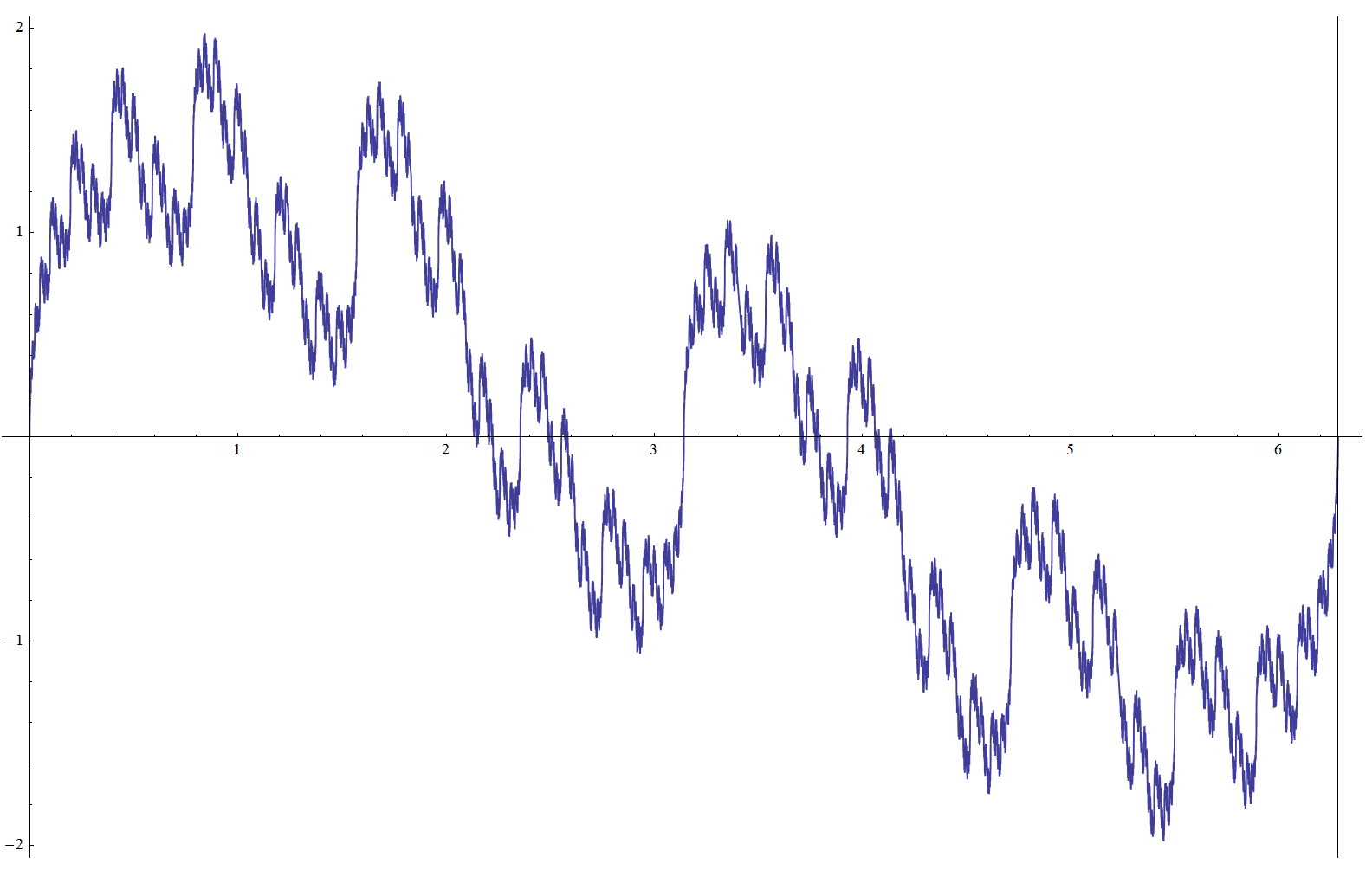
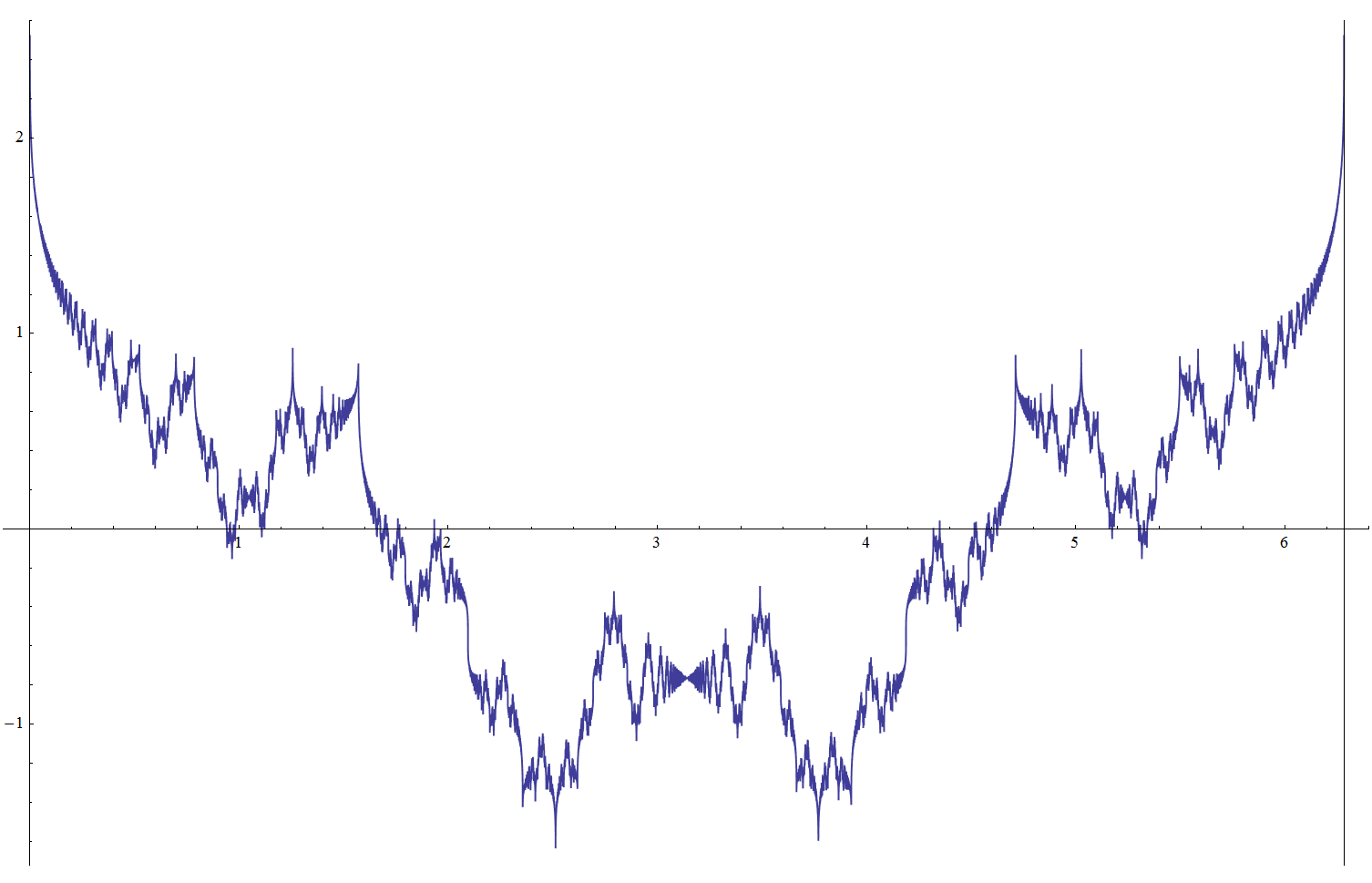
Weierstrass Sin and Cos functions, a = √2, b = 2, D = 3 / 2:

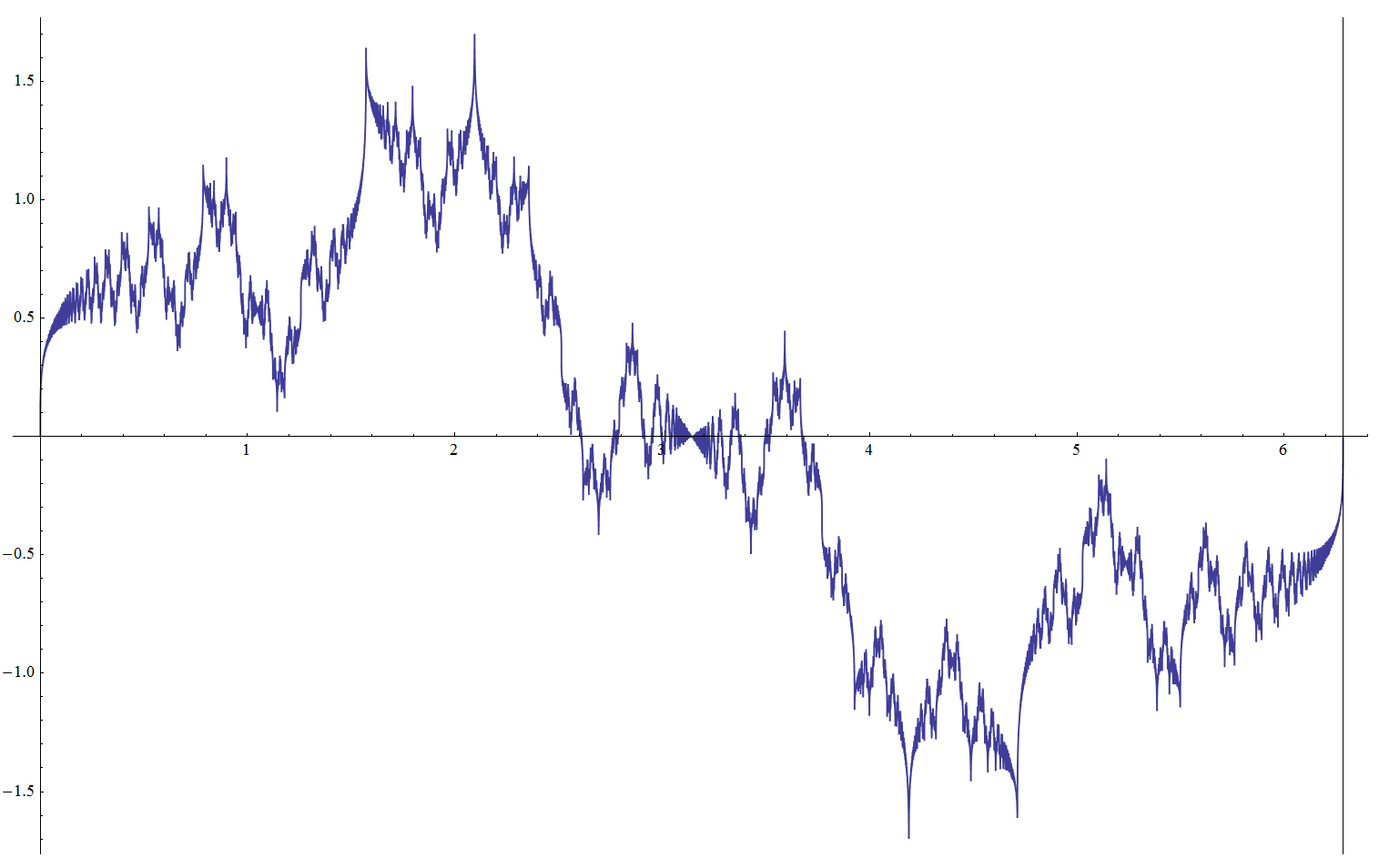
Riemann Sin and Cos functions, a = 3 / 2, b = 2, D = 3 / 2:
The sine and cosine versions can be viewed as the projections of a single complex-valued function F(t) = ∑ Ak Exp(i Fk t). If the frequency parameter is an integer, the function represents a closed curve on a complex plane.
N11 / Pawn protection of initial chess positions / #Math #Chess / 2015.08.01
Consider all possible arrangements of the chess pieces on the first rank. Assuming that the bishops occupy opposite-colored squares, there are 1440 reflection-distinct positions. 542 of these positions have every pawn protected at least once. Two maximally protected positions with only one pawn being protected once and all other pawns twice are RQBBRNKN and RKBBRNQN. Two minimally protected positions having three unprotected pawns are NNRQBKRB and NNRKBQRB.
The best overall position is apparently BQNRRNKB: the rooks are placed on the central files, the bishops on the main diagonals, each knight has four options for its first move, and only two pawns are protected just once.
N12 / Cantor's numbers / #Math / 2015.08.25
Recall Cantor's first uncountability proof. Start with an interval and a sequence of real numbers xi. Find the first two numbers from xi that lie inside the interval. These two numbers form the next interval. Repeat. In case of an infinite number of iterations, any number from the limit interval is not contained in xi.
Take a sequence of rational numbers within the initial interval, sorted in order of increasing denominator, and in case of equal denominators in order of increasing numerator. What number does Cantor's bracketing procedure converges to?
Take two fractions A = an / ad, B = bn / bd, ad ≤ bd, satisfying the determinant condition |bn ad - an bd| = 1. The first number lying between A and B is the mediant of A and B: M = (an + bn) / (ad + bd). The next number is the mediant of A and M. We thus obtain a system of recurrent equations:
ai = ai - 1 + bi - 1
bi = 2 ai - 1 + bi - 1
Thanks to the mediant property, the determinant condition is preserved throughout the recurrence. Eliminating bi gives a single recurrent equation ai + 1 = 2 ai + ai - 1, which has a solution ai = α (1 + √2)i + β (1 - √2)i. Plugging in initial conditions gives α = (a0 + b0 / √2) / 2. The sought-after Cantor number is the limit:
Lim ani / adi = αn / αd = (√2 an0 + bn0) / (√2 ad0 + bd0)N13 / Fraction digit tables / #Math / 2015.11.25
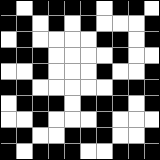
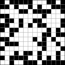
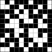
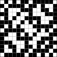
Following images depict binary and ternary digits of irreducible fractions in the (0, 1) interval. Fractions are ordered first by denominators and then by numerators.

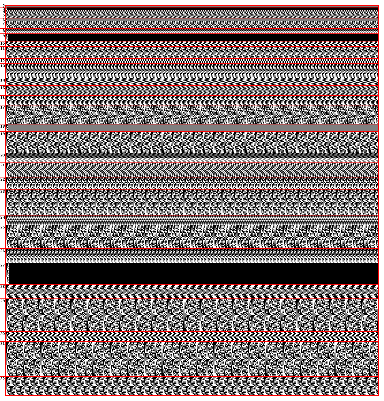
Take the numbers formed by digits lying on the main diagonal. By Cantor's diagonal argument, a complement of the binary diagonal number is irrational.
Binary diagonal number:Binary: 0.111000111001010110000110111110101011100111111011011010000100011 ... (OEIS A257341)
Decimal: 0.8890003549695230139346719690879129310538480210179543414543465370 ... (OEIS A257342)
Continued fraction: 0, 1, 8, 110, 1, 1, 1, 4, 1, 3, 33, 3, 4, 1, 26, 1, 37, 1, 23, 2, 117, 1, 1, 5, 1, 2, 20, 12, 1, 2, 1, 4, 1, ...
Ternary diagonal number:
Ternary: 0.1002211021120000111220000002000011111210202200100001202102121112 ...
Decimal: 0.3682120994629780785967399570406755660508922444001004151748993819 ...
Continued fraction: 0, 2, 1, 2, 1, 1, 12, 1, 2, 9, 2, 6, 5, 1, 2, 2, 7, 5, 1, 1, 2, 2, 2, 6, 7, 1, 41, 1, 4, 2, 2, 3, 1, ...
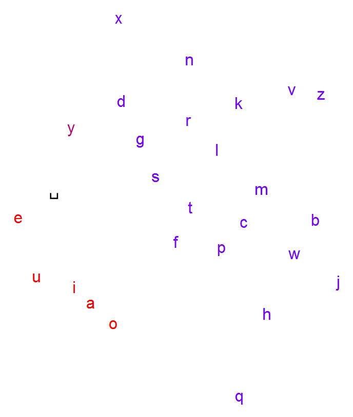
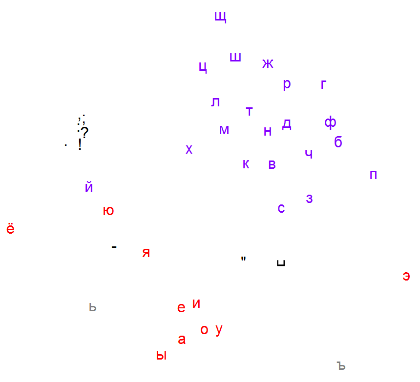
N14 / Multidimensional scaling for vowel-consonant separation / #Algorithms / 2015.12.04
Multidimensional scaling (MDS) can be effectively used for character-level text analysis. Denote the distribution of characters appearing at position δ relative to the character a as D(a, δ). Distance between characters a and b can be defined as
ρ(D(a, +1), D(b, +1)) + ρ(D(a, -1), D(b, -1)),where ρ(Da, Db) is some measure of distance between the two distributions. MDS applied to the distance matrices obtained from texts in natural languages readily reveals clusters of vowels, consonants and punctuation marks. Following images depict the results for English, Russian and Voynich manuscript characters and the L1 metric ρ.

N15 / Vectors with constant and normal components / #Math / 2016.01.29
Take a 2D vector having one constant component c and the other component coming from a standard normal distribution. PDF of the distribution of the vector lengths is given by ρ(x) = 2 x Exp(-(x2 - c2) / 2) / √τ (x2 - c2).
The mean of the distribution is approximated by √c2 + c / 6 + 4 / τ with a maximum relative error of 1%.
N16 / Embedding hexagonal grid in a square grid / #Programming #Board_Games / 2016.02.01
A subset of square grid locations (i, j) corresponding to a hexagonal grid is given by (i + 2 j) mod 4 = 0. Neighbours of a hex have offsets (0, ±2), (±2, ±1). 3D coordinates of a hex are
x = i / 2y = (-i + 2 j) / 4
z = (-i - 2 j) / 4
This representation is easy to work with, but has poor memory efficiency, as only 1/4th of all locations are actually used. However, these extra locations can be used to store additional information, for example serve as an intermediate buffer in a cellular automata scenario.
N17 / Irrationality plots / #Math / 2016.02.01
Let x be a real number, ai its continued fraction representation without the integer part, pi / qi its convergents. Let's define irrationality functions:
Fa = ∑ 2-i / ai
Fb = ∑ 1 / qi
Fc = ∑ 2-i Ln ai
For terminating continued fractions, ai is extended with +∞ terms, which does not changes the fraction value. Obviously Fa and Fb converge for all x. Fc converges almost everywhere except for rationals and some transcendentals with fast growing ai. Numerical calculations of Fc based on machine precision rationals should allways yeild +∞. So for the purpose of drawing Fc, ai is extended with Khinchin's constant representative of the typical ai values instead of +∞.
Fa(x):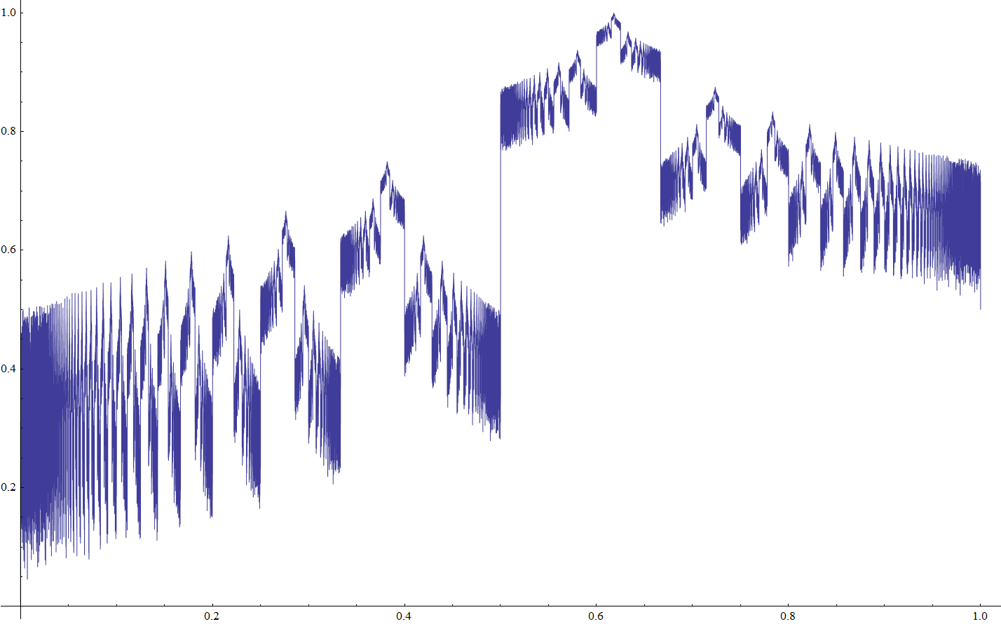
Fb(x):

Fc(x):

Local irrationality maxima are attained at x whose continued fractions end with an infinite sequence of 1s. Such x have Stern-Brocot tree paths that eventually alternate between left and right ad infinitum, as each run of left or right steps corresponds to a continued fraction term equal to its length. Take an interval [A, B], A = An / Ad, B = Bn / Bd with A, B being unimodular: |An Bd - Ad Bn| = 1. Suppose that B is the more complex fraction in a sense that Bd ≥ Ad and Bn ≥ An. This means that in the Stern-Brocot tree, B is a right child of A. Take the left step by computing a mediant of A and B, then the right step and so on. We thus obtain a system of recurrent equations for both numerators and denominators (see InvMem 12 for a similar recursion in a different context):
Axi + 1 = BxiBxi + 1 = Axi + Bxi
Solution to the above equations is a Fibonacci sequence:
Axi = α φi + β (-1 / φ)iα = (Ax0 + φ Bx0) / (1 + φ)
The sought-after limit, which might be called the golden mediant, is
Mg(A, B) = Lim An / Ad = (An + φ Bn) / (Ad + φ Bd)If A is the more complex fraction instead, A and B should be swapped before calculating the golden mediant. Mg(A, B) is a point of maximal irrationality on the unimodular interval [A, B]. Golden mediants share the worst rational approximation property (see Hurwitz's theorem) with the golden ratio.
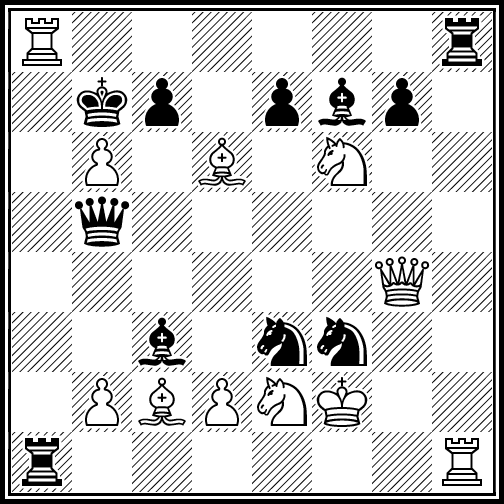
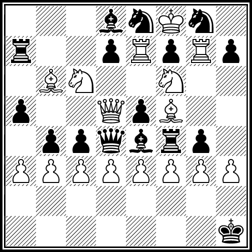
N18 / Maximal chess positions / #Chess #Optimization / 2016.02.04
Following record-breaking positions were generated with Ascension framework. Amount of improvement over the previous records (see "Guide to fairy chess" by Anthony Dickins) is indicated in brackets.

168 moves by both sides, all pieces on the board (+4)
183 moves by both sides, no promotions allowed (+2)
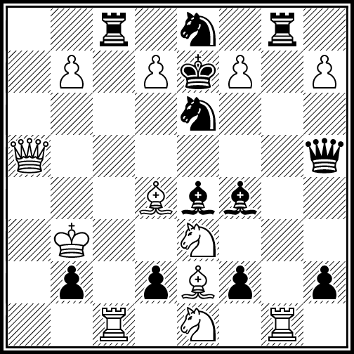
224 moves by both sides, promotions allowed (+1)
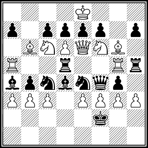
89 captures by both sides, all pieces on the board (+1)
50 captures by white, all pieces on the board (+1)
N19 / Weighted minimum and maximum / #Math / 2016.02.22
How can one define a weighted minimum and maximum of the numbers ai having weights wi? One approach is to calculate a limit of a weighted power mean:
WMax = Lim q√∑ a iq w iq / ∑ w ip, q → +∞ = Max(ai wi) / Max(wi)WMin = Lim q√∑ a iq w i-q / ∑ w i-q, q → -∞ = Min(ai / wi) / Min(1 / wi)
Another idea is to interpret the normalized weight wi as the probability of ai existing. Normalize the weights to unit maximum by dividing by Max wi . Sort ai in ascending | descending order. The probability of ai being the maximum | minimum is the probability of it existing and all greater | smaller values not existing:
pi = wi ∏ (1 - wj), j > i.The sought-after result is the mean of the resulting distribution: WMax | WMin = ∑ ai pi.
N20 / Maximal density subsquare-free arrangements / #Optimization #OpenProblem / 2016.02.22
What is the largest number of points that can be placed on a N × N grid so that no four of them form a square? Exact values are known for N up to 9 (OEIS A240443). Following solutions for N = 10 .. 16 were generated with tabu search and simulated annealing via Ascension framework.
 10: 50 | 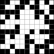 11: 58 | 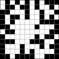 12: 67 | 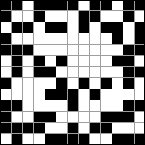 13: 76 |
 14: 86 | 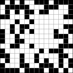 15: 95 | 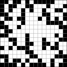 16: 106 |
If only axis-parallel squares are considered, maximal numbers are known for N up to 10 (OEIS A227133). Solutions obtained for N = 11 .. 16:
 11: 73 | 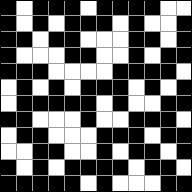 12: 85 | 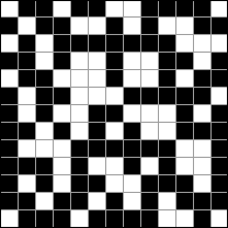 13: 98 |
 14: 112 |  15: 127 | 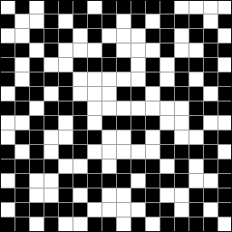 16: 142 |
N21 / Sierpinsky-like arrays / #Math / 2016.03.01
Define a 2 × 2 "seed" ((1, 1), (1, 0)). Start with A = ((1)), iteratively replace every element Aij with Aij × Seed. Resulting infinite array is essentially a Sierpinsky triangle. Alternatively, Aij can be defined as being equal to 1 only if binary representations of i and j do not contain a '1' in the same position: Aij = 1 if i AND j = 0, 0 otherwise, where AND denotes a bitwise 'and' operation.
Let a(n) = ∑ Aij for 0 ≤ i, j < n. a(2 n) = 3 a(n), because after a single replacement iteration, every 1 yields a block containing three new 1s. For odd indices, the edge contains incomplete blocks that only have two 1s, so a(2 n + 1) = 2 a(n + 1) + a(n) (A064194).
Two 3D versions arise naturally.
1. Seed = (((1, 1), (1, 1)), ((1, 1), (1, 0))). All three coordinates of nonzero elements never have a '1' bit in identical position: i AND j AND k = 0. Let a(n) = ∑ Aijk for 0 ≤ i, j, k < n. a(2 n) = 7 a(n). For odd n, in addition to incomplete 2 × 2 × 1 face blocks containing four 1s, there are 3 × 2Z(n) incomplete 2 × 1 × 1 edge blocks only containing two 1s, where Z(n) is the number of zeroes in the binary representation of n. Thus a(2 n + 1) = 4 a(n + 1) + 3 a(n) - 6 × 2Z(2 n + 1). a(n) (A269589) is a lower bound for the 3D verson of no subsquares problem (A268239, also see InvMem 20).
2. Seed = (((1, 1), (1, 0)), ((1, 0), (0, 0))). No pair of coordinates of nonzero elements contains a '1' bit in identical position: i AND j = 0, j AND k = 0, k AND i = 0. a(2 n) = 4 a(n), a(2 n + 1) = 3 a(n + 1) + a(n) (A268524).
N22 / Peaceable queens / #Math #Chess #Optimization / 2016.04.03
OEIS A250000 gives the largest M such that M white and M black queens can be placed on a N × N board and queens of opposite color do not attack each other. For N ≥ 14, simulated annealing yields solutions with 28, 32, 37, 42, 47, 52, 58, 64, 70, 77, 84 queens per side.
Solutions typically consist of four polygonal regions. What happens at the limit N → ∞? Replace the N × N board by a unit square. The areas of the regions (see illustration) are:
A2 = (1 − 4 x2 − 2 y2) / 8
A = A1 + A2 = (2 x (1 − 2 x) + y (2 − 3 y)) / 4
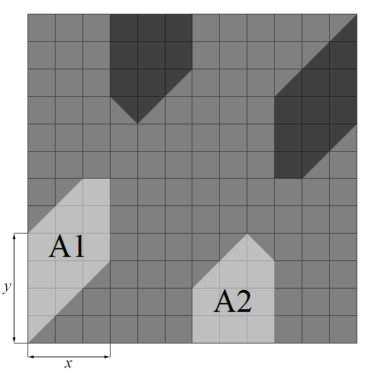
Maximum of the total area A is 7 / 48, attained at x = 1 / 4, y = 1 / 3. Observation: with a few exceptions having a non-polygonal structure (N = 5, 9), M = Floor(7 / 48 N2).
N23 / RGB Principal component analysis / #Math #Color / 2016.05.29
Principal component analysis applied to gamma-compressed RGB values from a large set of photographic images (MIRFLICKR25000 dataset) yielded the following transformation matrix:
| 0.576 | 0.585 | 0.571 |
| 0.721 | -0.034 | -0.692 |
| -0.386 | 0.810 | -0.441 |
Relative importance of the axes, as measured by the square root of their eigenvalues, is about 1 : 1/3 : 1/7. The axes closely correspond to black - white, orange - azure (hue 30° - 210°) and green - magenta (hue 120° - 300°) directions. Normalized to unit dynamic range of the axis projections, the matrix is well approximated by
| 1/3 | 1/3 | 1/3 |
| 1/2 | 0 | -1/2 |
| -1/4 | 1/2 | -1/4 |
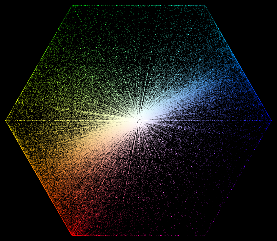
Projection of the RGB values
normalized to unit maximum
along the main cube diagonal
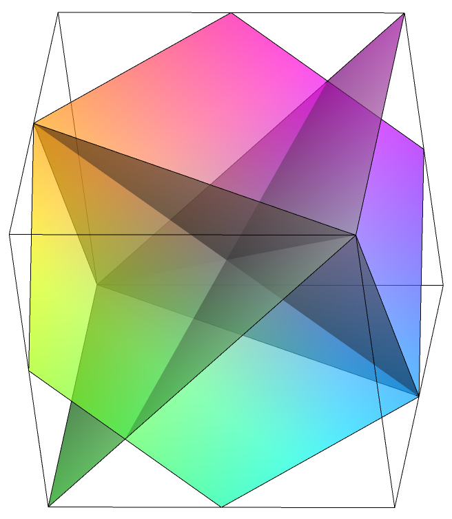
Approximate PCA planes
N24 / Lightness approximations / #Color #Approximation / 2016.05.29
Lightness of a color can be calculated with the aid of the Lab color system, but in many cases a simple approximation would suffice. Following tables summarize such approximations. R, G, B denote gamma-compressed sRGB values. Equivalent gray level denotes the level of sRGB gray having the same lightness as the color in question. The approximations were obtained by minimizing the L2 and L∞ errors. L2 error is weighted with typical real-world colors (RGB data taken from the MIRFLICKR25000 dataset), and the L∞ error was calculated along the whole RGB cube. All the approximations give 0 when applied to black and 1 when applied to white.
| Equivalent gray level approximation | Error | |
| 0.301 R + 0.622 G + 0.077 B | L2 = | 1 / 55 |
| 0.279 R + 0.643 G + 0.078 B | L∞ < | 1 / 4 |
| (0.228 R2 + 0.696 G2 + 0.076 B2)1 / 2 | L2 = | 1 / 367 |
| (0.224 R2 + 0.700 G2 + 0.076 B2)1 / 2 | L∞ < | 1 / 38 |
| (0.215 Rp + 0.714 Gp + 0.071 Bp)1 / p, p = 2.169 | L2 = | 1 / 496 |
| (0.234 Rp + 0.695 Gp + 0.071 Bp)1 / p, p = 2.063 | L∞ < | 1 / 40 |
| Lightness approximation | Error | |
| 0.325 R + 0.641 G + 0.034 B | L2 = | 1 / 30 |
| 0.288 R + 0.633 G + 0.079 B | L∞ < | 1 / 4 |
| (0.267 R2 + 0.674 G2 + 0.059 B2)1 / 2 | L2 = | 1 / 43 |
| (0.232 R2 + 0.692 G2 + 0.076 B2)1 / 2 | L∞ < | 1 / 19 |
| (0.208 Rp + 0.744 Gp + 0.048 Bp)1 / p, p = 2.909 | L2 = | 1 / 47 |
| (0.222 Rp + 0.705 Gp + 0.073 Bp)1 / p, p = 2.134 | L∞ < | 1 / 24 |
| (0.213 Rp + 0.730 Gp + 0.057 Bp)1 / q, p = 2.211, q = 2.367 | L2 = | 1 / 76 |
N25 / Feature scaling / #Math / 2016.10.15
Feature scaling directly affects the results of dimensionality reduction methods such as PCA and MDS. Standardization (rescaling to zero mean and unit variance) is the most common method. But if all the features belong to a ratio scale (have a meaningful zero), one can divide by the mean or the root mean square instead.
| Normalization factor | Feature importance |
|---|---|
| 1 | σ |
| σ | 1 |
| μ | CV |
| √⟨x2⟩ | CV / √1 + CV2 |
A feature's impact is proportional to its standard deviation after the normalization. Standardization assigns equal importance to all features, while the unit mean and RMS normalization emphasize features with a higher coefficient of variation (CV = σ / μ), which may be more appropriate if relative differences are important. Note that the RMS normalization guarantees bounded feature importance. If all the features have the same units of measurement, the normalization can be skipped, although it would likely be beneficial if the features significantly differ in scale.
Another potential issue is the presence of highly correlated features. Duplicating a feature adds no new information but will distort the results of PCA or MDS. Consider a dataset having D uncorrelated features. Replace each feature i by Mi duplicates. The data will now lie in a subspace spanned by D oblique axes and each feature will be inflated by a factor of √Mi.
Collinear inflation correction (CIC) factors applicable in the general case have the form Fi = √∑ Corr2(i, j), where Corr(i, j) is Pearson's correlation between features i and j. CIC provides a principled and robust alternative to discarding highly correlated features. It is independent of the feature normalization and should be performed in conjunction with it.
N26 / Mixed radix fractal carpets / #Math / 2017.04.18
Sierpinski carpet can be constructed from a single cell by iteratively subdividing the grid into 3 x 3 cell blocks and then removing the cells with both coordinates equal to 1 modulo 3. If 2 is used in place of 3, the procedure would yield a Sierpinski triangle. However, the subdivision factor S and the coordinate test modulo M need not necessarily be the same. Let's call such cases mixed radix carpets (or (hyper)sponges, depending on the dimension).
The total number of cells in a mixed radix carpet at iteration i can be calculated by considering the numbers of cells with various values of coordinates modulo M. Denote by (x; y; ...) the cells with coordinates modulo M identical to x, y, ... up to a permutation, and by N(x; y; ...) the number of such cells. Let's examine the case S = 3, M = 2 and the cells (1; 1) being excluded. Subdivision produces the following cells:
(0; 0) → 4(0; 0), 4(0; 1), 1(1; 1)(0; 1) → 2(0; 0), 5(0; 1), 2(1; 1)
(1; 1) → 1(0; 0), 4(0; 1), 4(1; 1)
Since the cells (1; 1) are excluded, at iteration i + 1 we have:
Ni + 1(0; 0) = 4 Ni(0; 0) + 2 Ni(0; 1)Ni + 1(0; 1) = 4 Ni(0; 0) + 5 Ni(0; 1)
The total number of cells Ni + 1 = 8 Ni(0; 0) + 7 Ni(0; 1). By substitution, Ni + 2 = 60 Ni(0; 0) + 51 Ni(0; 1), and through simple algebraic manipulations we obtain Ni + 1 = 9 Ni − 12 Ni − 1. Asymptotic growth rate is the largest root of the characteristic polynomial: R = (9 + √33) / 2, and the fractal dimension is D = Ln R / Ln S.
Results for other values of S, M and other dimensions can be obtained in the same manner. In general, the system of linear recurrence equation is defined by the subdivision matrix with rows and columns corresponding to the excluded cells removed. Here are two more subdivision rules in matrix form:
| 3D, S = 3, M = 2: | (N(0; 0; 0), N(0; 0; 1), N(0; 1; 1), N(1; 1; 1)) · |
|
| 2D, S = 2, M = 3: | (N(0; 0), N(0; 1), N(1; 1), N(0; 2), N(2; 2), N(1; 2)) · |
|
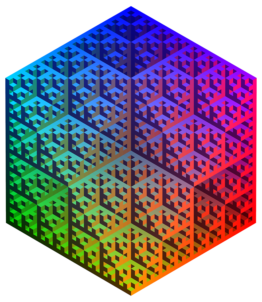
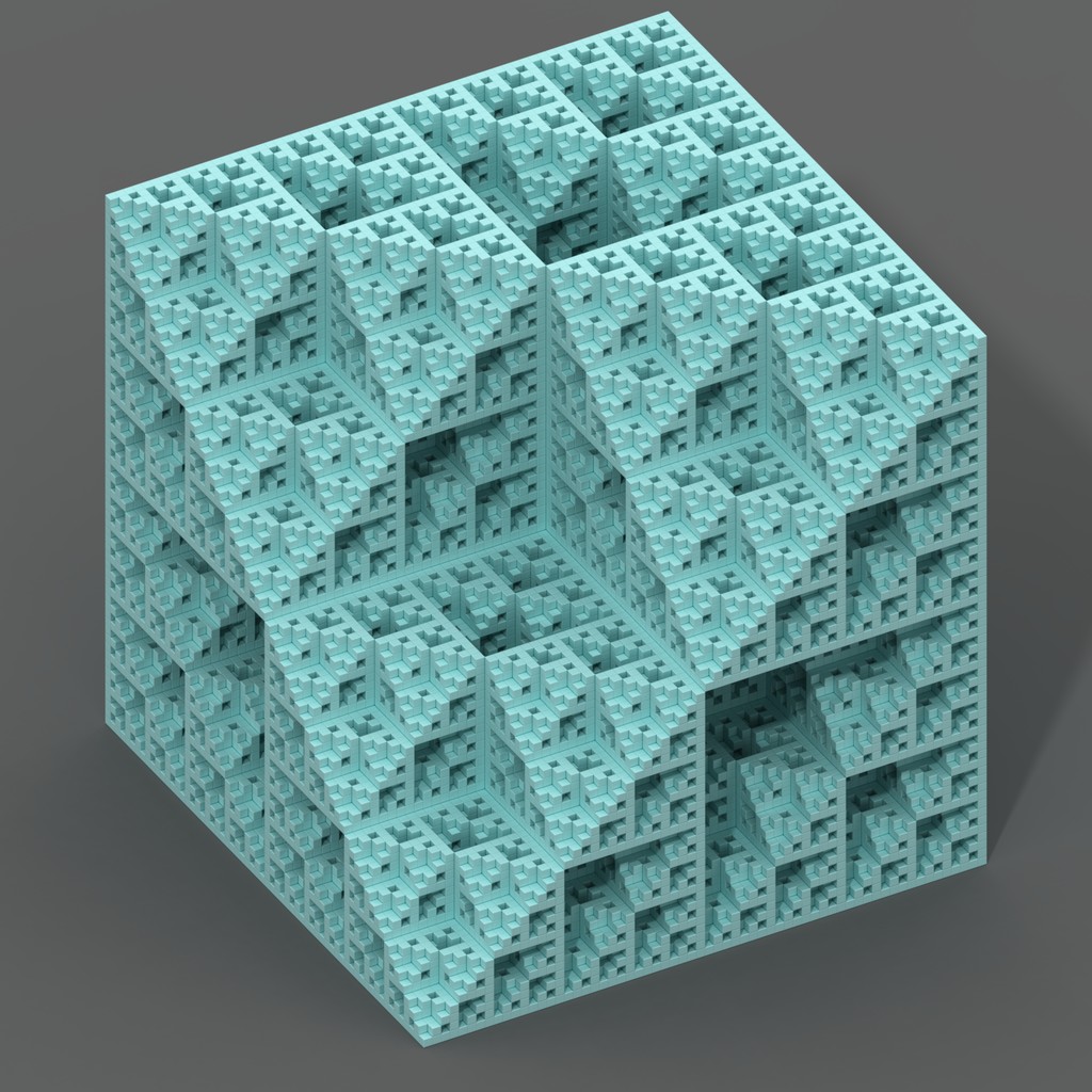
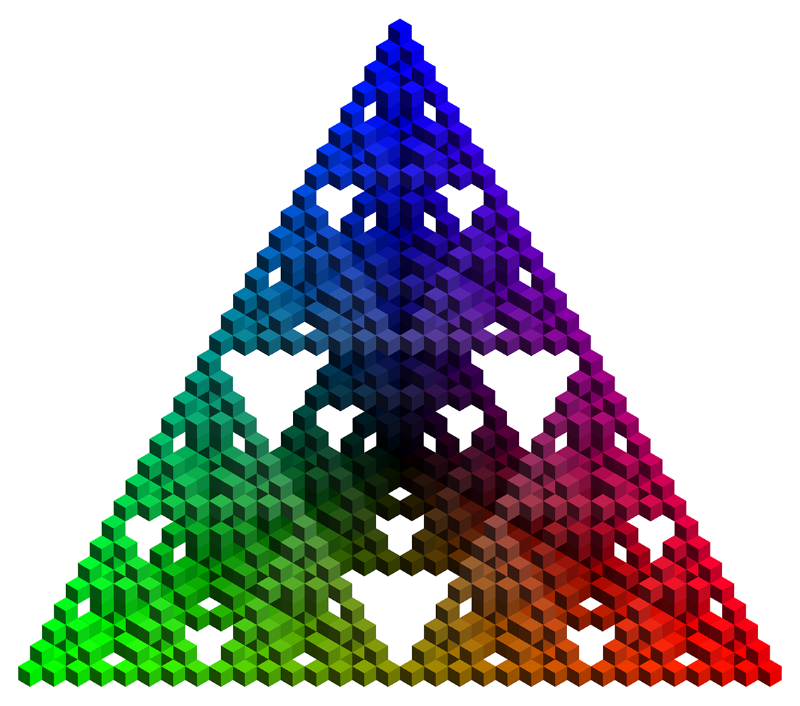
Results for selected cases are summarized in the following table. D0 is the grid dimension; excluded cells are denoted by the number of '1's in their coordinates modulo M.
| S | M | D0 | Excluded | Recurrence | R | D | First terms | OEIS | Images |
|---|---|---|---|---|---|---|---|---|---|
| 2 | 3 | 2 | 0 | 2 | 2 | 1 | 1, 3, 4, 8, 16, 32, 64, 128, ... | A000079, i > 1 | 8 |
| 2 | 3 | 2 | 0, 2 | 2 | 2 | 1 | 1, 2, 4, 8, 16, 32, 64, 128, ... | A000079 | 8 |
| 2 | 3 | 2 | 1 | 1, 4 | 2.562 | 1.357 | 1, 2, 6, 14, 38, 94, 246, 622, ... | A026597 | 8 |
| 2 | 3 | 2 | 2 | 3, 2 | 3.562 | 1.833 | 1, 3, 11, 39, 139, 495, 1763, ... | A007482 | 8 |
| 3 | 2 | 2 | 1, 2 | 4 | 4 | 1.262 | 1, 4, 16, 64, 256, 1024, ... | A000302 | 5 |
| 3 | 2 | 2 | 0, 1 | 4 | 4 | 1.262 | 1, 1, 4, 16, 64, 256, 1024, ... | A000302, i > 0 | 5 |
| 3 | 2 | 2 | 1 | 5 | 5 | 1.465 | 1, 5, 25, 125, 625, 3125, ... | A000351 | 5 |
| 3 | 2 | 2 | 0, 2 | 5 | 5 | 1.465 | 1, 4, 20, 100, 500, 2500, ... | A005054 | 5 |
| 3 | 2 | 2 | 2 | 9, −12 | 7.372 | 1.818 | 1, 8, 60, 444, 3276, 24156, ... | A285391 | 5 |
| 3 | 2 | 2 | 0 | 9, −12 | 7.372 | 1.818 | 1, 5, 36, 264, 1944, 14328, ... | A285392 | 5 |
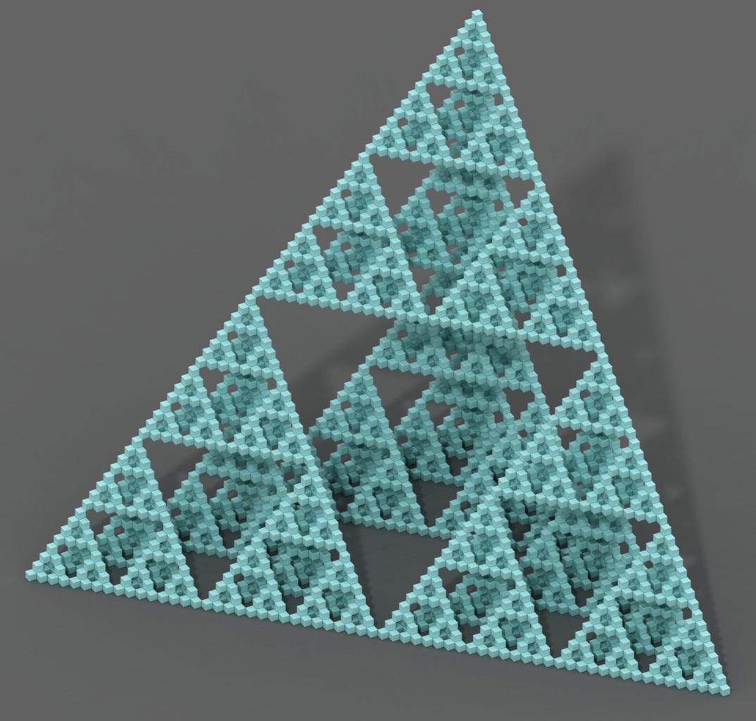
| 3 | 2 | 3 | 1, 2, 3 | 8 | 8 | 1.893 | 1, 8, 64, 512, 4096, 32768, ... | A001018 | 1, 2, 3, 4 |
| 3 | 2 | 3 | 0, 1, 2 | 8 | 8 | 1.893 | 1, 1, 8, 64, 512, 4096, ... | A001018, i > 0 | 1, 2, 3, 4 |
| 3 | 2 | 3 | 1, 2 | 9 | 9 | 2 | 1, 9, 81, 729, 6561, 59049, ... | A001019 | 1, 2, 3, 4 |
| 3 | 2 | 3 | 0, 2, 3 | 12 | 12 | 2.262 | 1, 12, 144, 1728, 20736, ... | A001021 | 1, 2, 3, 4 |
| 3 | 2 | 3 | 0, 1, 3 | 12 | 12 | 2.262 | 1, 6, 72, 864, 10368, ... | A067419 | 1, 2, 3, 4 |
| 3 | 2 | 3 | 1, 3 | 14 | 14 | 2.402 | 1, 14, 196, 2744, 38416, ... | A001023 | 1, 2, 3, 4 |
| 3 | 2 | 3 | 0, 2 | 14 | 14 | 2.402 | 1, 13, 182, 2548, 35672, ... | A285399 | 1, 2, 3, 4 |
| 3 | 2 | 3 | 2, 3 | 20, −48 | 17.211 | 2.590 | 1, 20, 352, 6080, 104704, ... | A285393 | 1, 2, 3, 4 |
| 3 | 2 | 3 | 0, 1 | 20, −48 | 17.211 | 2.590 | 1, 7, 116, 1984, 34112, ... | A285394 | 1, 2, 3, 4 |
| 3 | 2 | 3 | 2 | 28, −195, 324 | 18.322 | 2.647 | 1, 21, 399, 7401, 136227, ... | A285396 | 1, 2, 3, 4 |
| 3 | 2 | 3 | 1 | 28, −195, 324 | 18.322 | 2.647 | 1, 15, 249, 4371, 78693, ... | A285395 | 1, 2, 3, 4 |
| 3 | 2 | 3 | 0, 3 | 21 | 21 | 2.771 | 1, 18, 378, 7938, 166698, ... | A285400 | 1, 2, 3, 4 |
| 3 | 2 | 3 | 3 | 32, −195, 216 | 24.359 | 2.906 | 1, 26, 646, 15818, 385822, ... | A285397 | 4 |
| 3 | 2 | 3 | 0 | 32, −195, 216 | 24.359 | 2.906 | 1, 19, 452, 10948, 266300 ... | A285398 | 1, 2, 3, 4 |
N27 / Random strings with identical element counts / #Math / 2018.05.31
Probability of two random binary strings of length n having identical bit counts is
P = ∑0 ≤ i, j ≤ n, i + j = n ((i, j)! / 2n)2 = (n, n)! / 4n = A000984 / 4n = √2 / τ (n − 1/2)! / n! ≈ 1 / √6 / 7 + τ n / 2Probability of two random ternary strings having identical element counts is
P = ∑0 ≤ i, j, k ≤ n, i + j + k = n ((i, j, k)! / 3n)2 = A002893 / 9n ≈ 1 / (4 / 7 + (2 τ / 33/2) n),where (a, b, c, ...)! = (a + b + c + ...)! / (a! b! c! ...) is the multinomial coefficient.
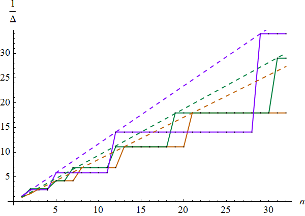
N28 / Irrational scoring / #Math / 2018.05.31
Irrational point system can be employed to eliminate the possibility of several players having an equal score in a tournament unless their numbers of wins and draws are identical. Due to worst rational approximation properties (Hurwitz's theorem), suitable choices for the win / draw point ratio are 1 + φ, 4 − φ and γ, where φ = (1 + √5) / 2 is the golden ratio and γ = 1 + √2 is the silver ratio. These values result in the following dependencies of the minimal gap between two different scores Δ on the number of games n:
| Win / draw ratio | Asymptotic worst case Δ | Worst case n |
|---|---|---|
| 1 + φ | (1 + φ) / (√5 n) ≈ 1.17 / n | 2, 3, 5, 8, 13, 21, 34, ... (A000045) |
| 4 − φ | (4 − φ) / (√5 n) ≈ 1.07 / n | 2, 5, 7, 12, 19, 31, 50, ... (A013655) |
| γ | γ / (√8 n) ≈ 0.85 / n | 2, 5, 12, 29, 70, 169, 408, ... (A000129) |
N29 / Correlation for vector-valued data / #Math / 2018.05.31
Pearson's correlation coefficient can be extended to vector-valued data by replacing multiplication with a dot product. In other words, correlation is the mean dot product between the corresponding elements of the datasets normalized to zero mean and unit mean square vector length.
If you appreciate the effort put into creating this page and would like to see more frequent updates, you can support me on Patreon. Top patrons of the month:
- Brian Bucklew
- Anton Shepelev
- Adam Hill
- Tomoyuki Naito
- John Metcalf