Contents
IntroductionTesting methodology
Rainbow map
Cubehelix
Matplotlib
Other
Proposed designs
List of all tested colormaps
Statistics
References
Introduction
Using a colormap instead of a grayscale palette for data visualization can help convey more information. On the other hand, a poor colormap can misrepresent the data and make the interpretation difficult. In this post, I examine various linear (intended for real-valued data) colormaps and introduce a few novel ones.
Change of hue in addition to lightness provides a complimentary way to estimate the value of the datum. It is, therefore, important for a colormap to have a wide hue range and a reasonably high saturation. But while providing additional information, the colormap should not distort the data. Let's define the resolution as the smallest detectable data difference. An ideal colormap should be perceptually-uniform - that is, have a constant resolution across its whole range. Lightness uniformity (a constant increase of the perceived lightness) is also important, as it allows safe grayscale conversion. The informativity and faithfulness of representation requirements are hard to reconcile, making the colormap design problem inherently difficult.
Summary of colormap criteria:
- Informativity
- Wide lightness range
- Wide hue range
- Saturation not too low
- High minimal resolution
- Faithfulness
- Lightness uniformity
- Perceptual uniformity
- Smoothness: no abrupt color bands or sharp transitions
- Aesthetics
- Should not contain unpleasant color combinations
Testing methodology
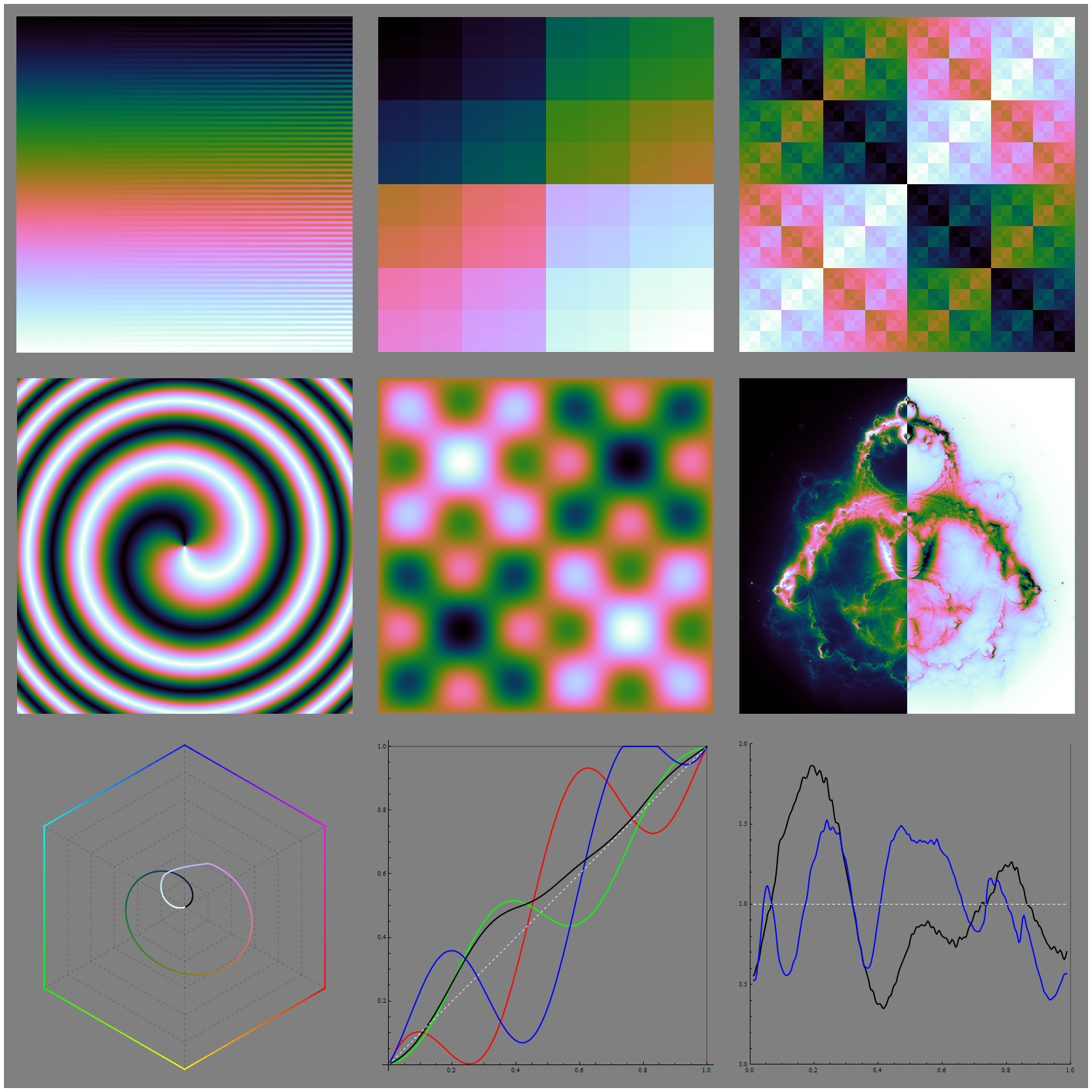
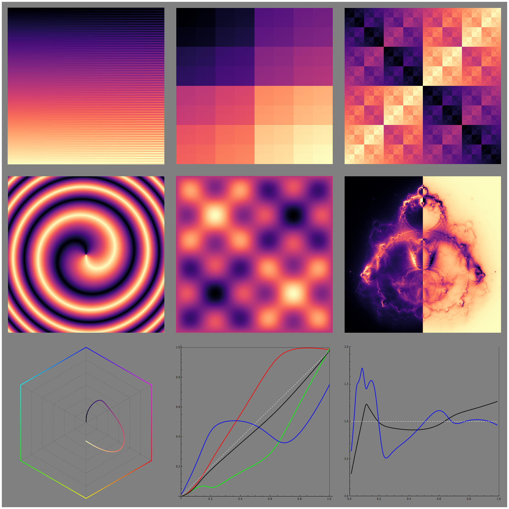
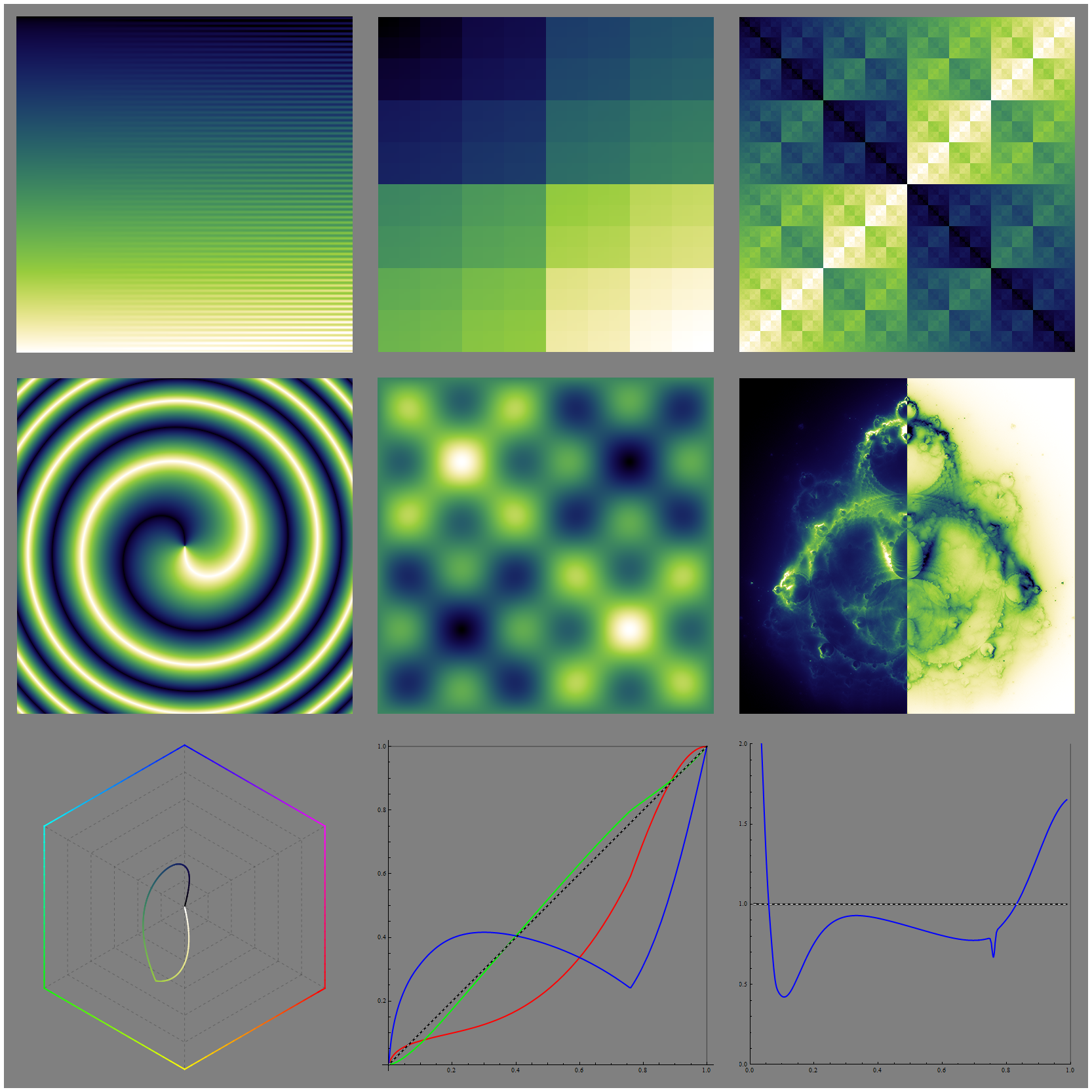
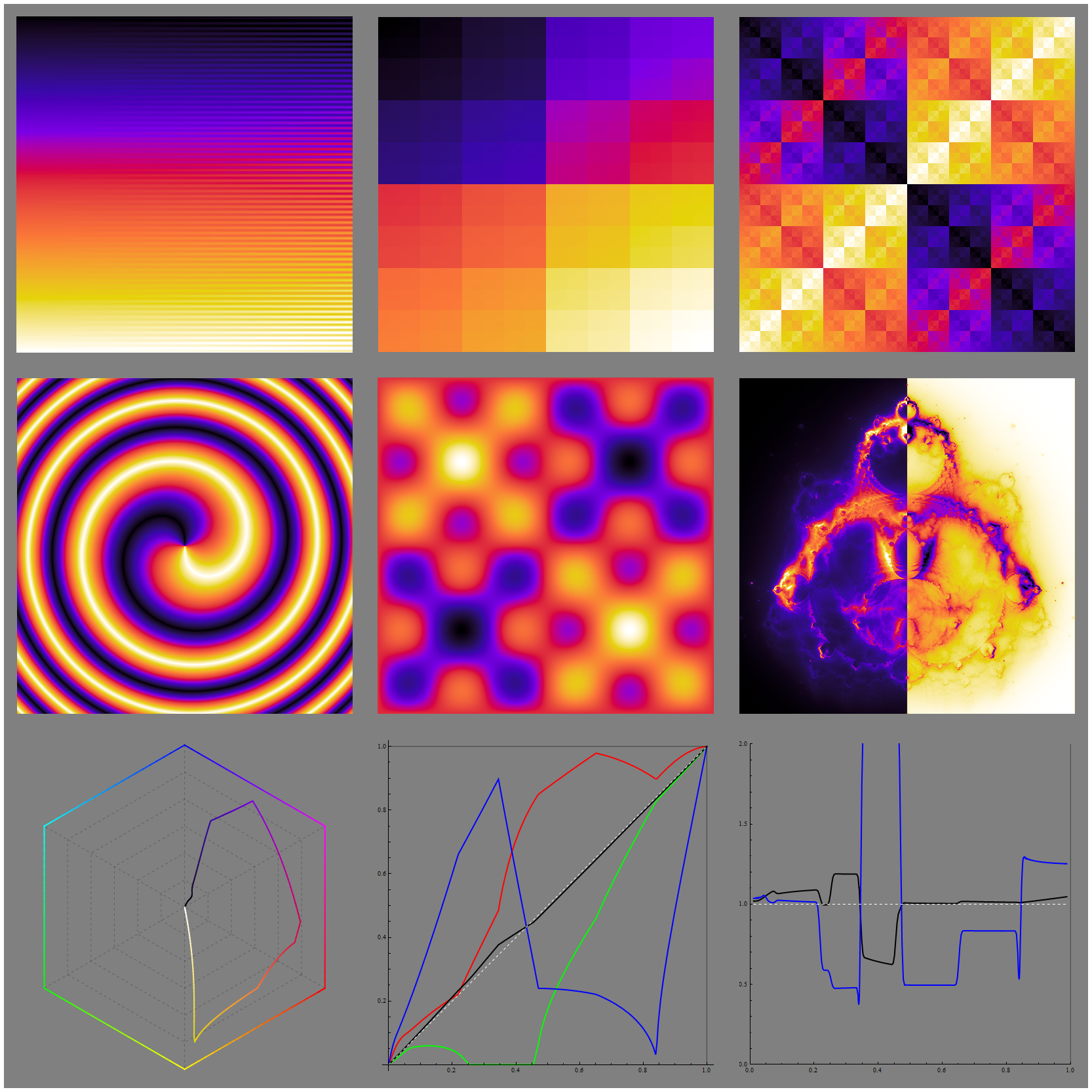
To test various colormap criteria, I came up with 6 test images:
- Ramp: W(x, y) = y + x2 Sin(64 τ y) / 12, clipped into [0, 1] interval. Slightly modified version of the test function introduced by Peter Kovesi [1]. Allows to visually assess perceptual uniformity by observing the distance at which the sine pattern fades.
- Z-Order: W(i, j) is constructed by interleaving the bits of j and i. A good color map should be able to resolve 4 subsquares within each of the 16 squares. The difference along the edge of the vertically adjacent subsquares is 1/48 and along the edge of the horizontally adjacent ones is 1/96 of the full range.
- Xor: W(i, j) = Bitwise xor of i and j, 0 ≤ i, j ≤ 511. Another resolution test. A good colormap should be able to resolve the contents of any 32x32-pixel subsquare (1/16 of the data range).
- Spiral: W(x, y) = ArcSin(Sin(2 τ (x2 + y2) + ArcTan(x, y))), -1 ≤ x, y ≤ 1. Smoothness test, has a near-uniform distribution of values.
- Two sine products: W(x, y) = Sin(x) Sin(y) + Sin(3 x) Sin(3 y), -τ/2 ≤ x, y ≤ τ/2. Smoothness test.
- Buddhabrot fractal (1000 iterations) with one half inverted, courtesy of Wikipedia. Represents the case when the data is dominated by either the lowest or the highest values.
- Projection of the colormap path through the RGB space along the main diagonal
- Plot of R, G, B and lightness components
- Lightness and Lab uniformity (L and Lab derivatives, black and blue respectively)
Perceived lightness is fairly well approximated by the L component of the Lab color system, so the lightness uniformity function can be obtained by taking the derivative of L. In theory, the perceptual uniformity can be calculated by taking a derivative of the colormap in a perceptually uniform colorspace such as Lab. But I found that the norm of the Lab derivative correlates poorly with the perceived resolution. Peter Kovesi asserts [1] that at high spatial frequencies, the perceptual uniformity is dominated by the lightness uniformity. In my experience, while most of the time this is the case, certain colors can cause noticeable deviations. Therefore the best way to test the perceptual uniformity is to use the test images.
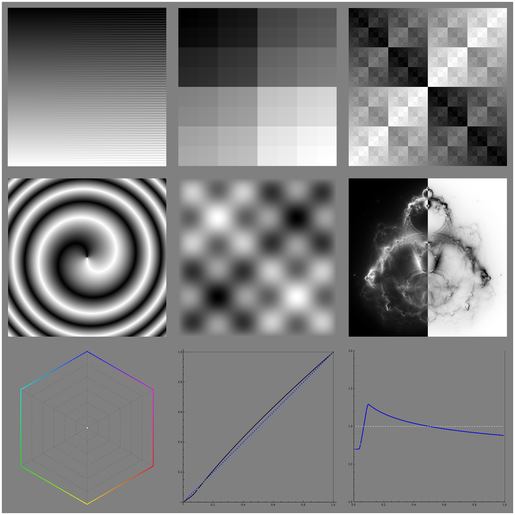
It is assumed that all the colormaps take a unit range variable t as an argument, and all the data are also rescaled into the unit range. Y coordinate of all the test images goes from top to bottom. To avoid distortions, the test image should be viewed in 1:1 scale (2:1 if you have an ultra-HD display). Here is a test of the baseline [lightness-uniform grayscale map] (not to be confused with the [RGB-uniform grayscale]). I did not perform any kind of separate color-blind testing because being deuteranopic, I have this feature built in. Your eyesight and hardware will likely differ, so you are free to come up with your own conclusions.
Rainbow map
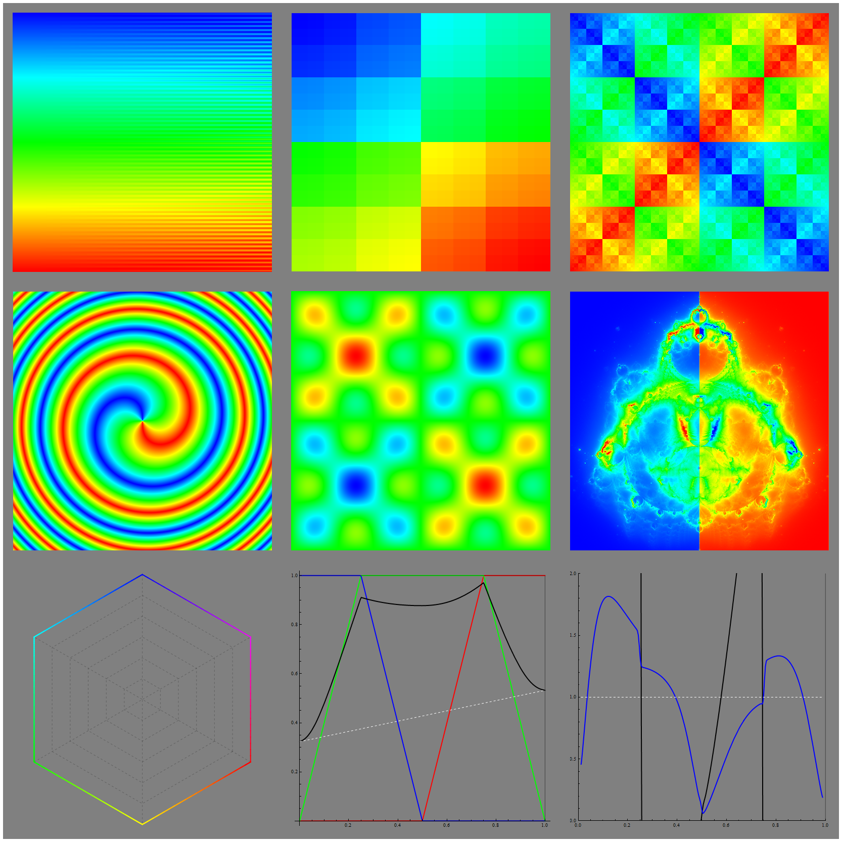
[HSV rainbow map] is defined by HSV coordinates (240 ° − 240 ° t, 1, 1) - in other words, it goes from blue to red through colors of maximal intensity. Much has been said about its perils [2, 3], but a test image is worth a thousand words.
The map satisfies the informativity criteria, having a large hue range and maximal saturation, but fails badly the faithfulness counterpart. First, its lightness profile is non-monotonic and it has two prominent color bands at cyan and yellow. This results in heavy distortions of whatever data you are trying to visualize. Second, the resolution in the cyan-green region is absolutely terrible, dropping as low as 1 / 9 of the data range! In short, if you use the rainbow map, good luck interpreting your data.
Various software vendors supply their own versions of the rainbow map (Matlab's jet, Mathematica's "Rainbow"), but all of them share the same core problems. Matteo Niccoli's blog details his attempts to fix the rainbow map by making it more lightness-uniform. Here is one of the maps he provides, [cubeYF]. The lightness profile is monotonically increasing (although nonlinear), and the ugly banding is gone. The main problem is very poor resolution pretty much everywhere after the first 5 z-squares. Another map is a [linear L rainbow]. While being a huge improvement over the basic rainbow map (and over the Kindlmann version [4]), unfortunately, it has some banding issues. There is a strange L glitch and a tiny green band at t = 0.6, and the yellow-white transition looks abrupt and unnatural.
Cubehelix
Cubehelix [5] is a family of colormaps that go from black to white through a helix in the RGB space. Starting hue, number of rotations, saturation and a skew parameter specify a particular colormap. Despite the author's intention, Cubehelix is not lightness-uniform, as it relies on luma approximation. The most noticeable consequence is a loss of resolution near t = 0.
The author provides the [default settings], but they aren't very good. There is a significant loss of resolution near violet (t = 0.72) and the green-magenta combination is aesthetically dubious (a study of color harmony [6] identifies it as the most displeasing one). The saturation is rather poor but when it is increased, the colormap turns from not very good to downright hideous [hue = 1.5].
These issues are caused by a large number of turns. No matter what the starting hue is, 1.5 turns lead to problematic transitions appearing at some point. [Single-turn settings] proposed in the If We Assume blog are a significant improvement over the defaults. By further reducing the number of turns down to 2/3 it becomes possible to safely increase the saturation. Here are some of the better Cubehelix parameters I was able to find:
[start: 1.0, rotations: -1, hue: 1.0]
[start: 0.25, rotations: -0.67, hue: 1.5]
[start: 0.75, rotations: -0.67, hue: 1.5]
Matplotlib
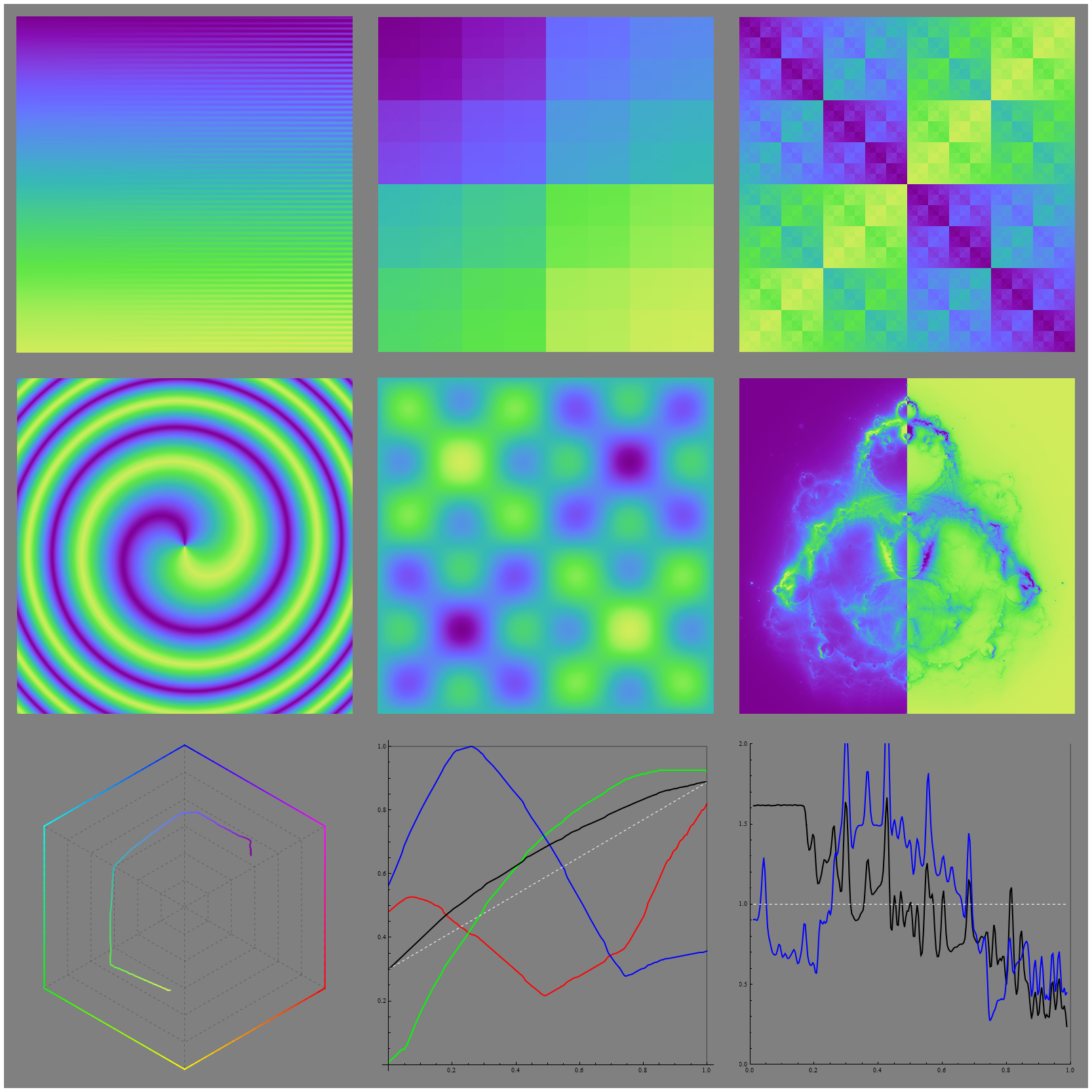
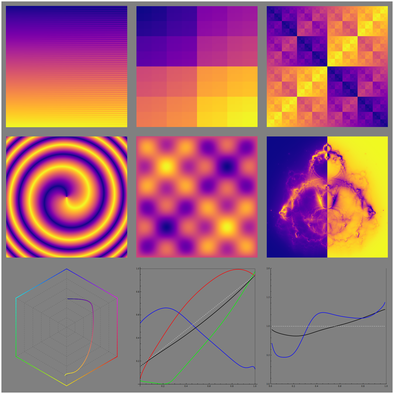
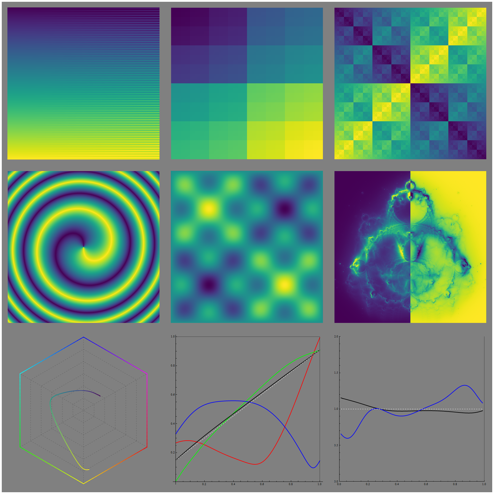
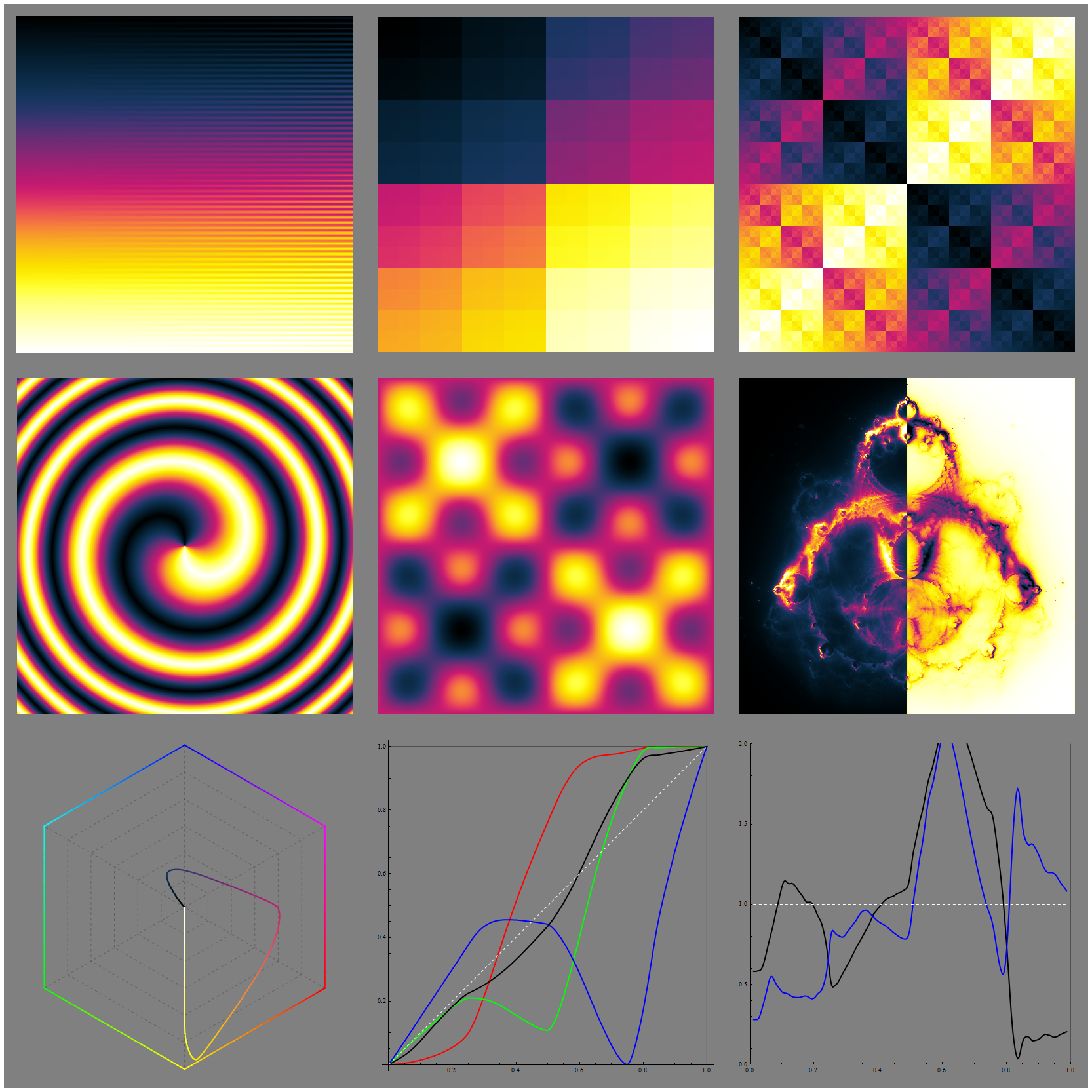
Matplotlib colormaps [Magma, Inferno, Plasma, Viridis] rely on the advanced CAM02-UCS colorspace to achieve perceptual and lightness uniformity. However, Magma and Inferno have pitch-black first z-square - a far cry from uniformity of any kind. Plasma and Viridis avoid this problem, but have a reduced lightness range. Viridis was selected by popular vote as the default Matplotlib colormap, but I am not impressed by it, as the reduced lightness range coupled with a particular choice of colors results in a comparatively poor overall contrast. This leaves Plasma as the only Matplotlib option which I don't have a problem with.
Other
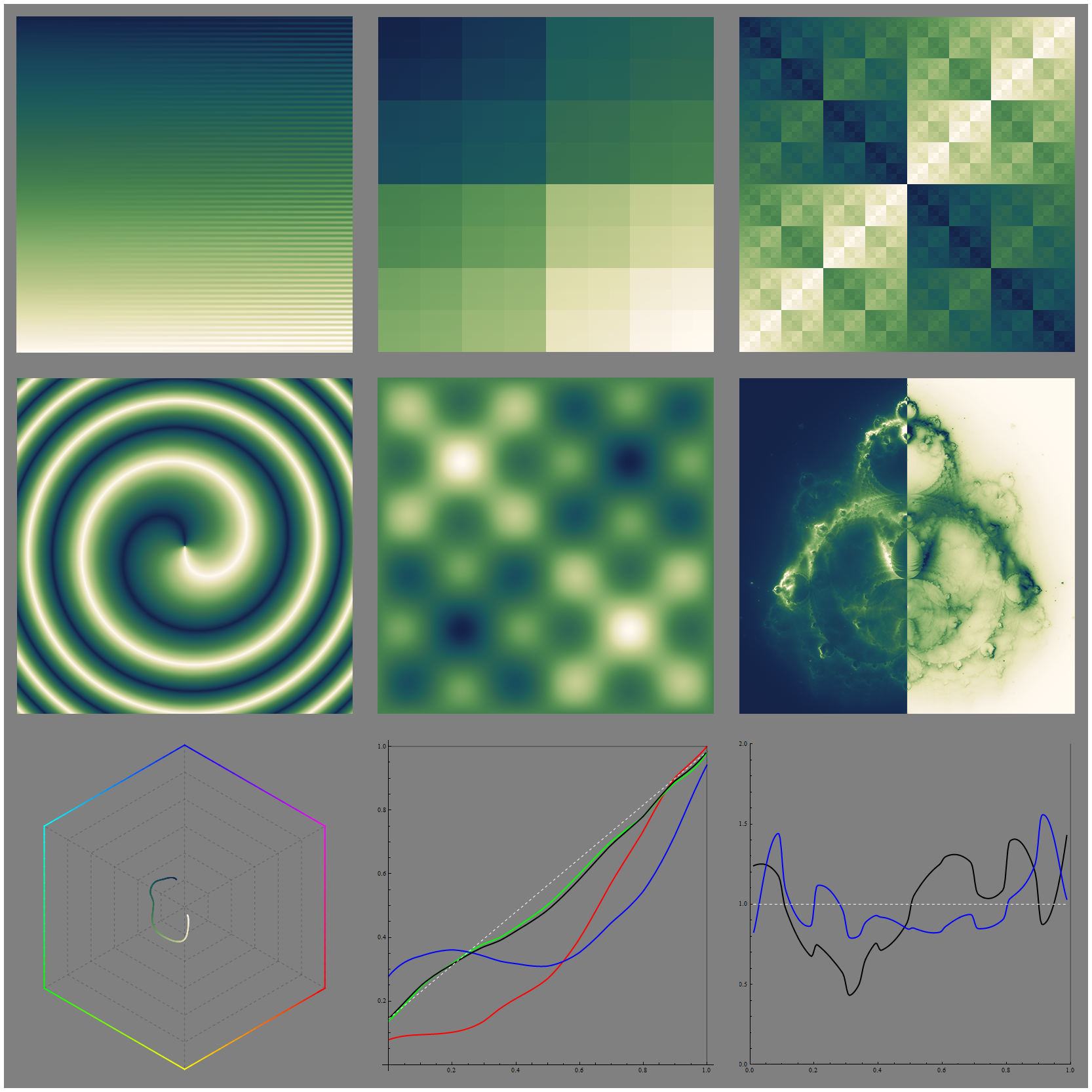
Peter Kovesi's colormaps [1] are constructed with the aid of perceptual contrast equalization process that ensures lightness uniformity. Most of them fail either the lightness range, hue range or smoothness criteria, so I've only selected two of them: [KRYW, BGYW].
A number of linear colormaps are available from the Los Alamos National Laboratory website, but almost all of them are monochromatic. The most informationally dense-looking one is [Olive Green to Blue] (reversed for consistency).
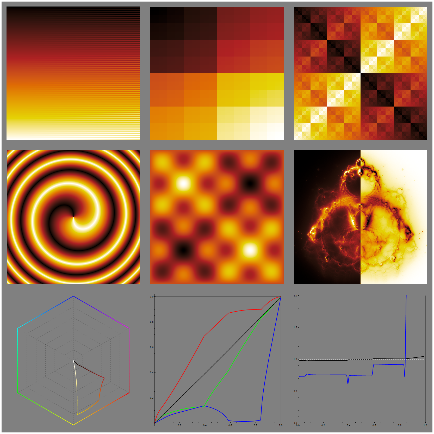
Kenneth Moreland provides a couple of lightness-unform colormaps, [Black Body] and [Extended Black Body]. Note the awkward yellow-white transition. The extended version tries to improve upon the narrow hue range of its red-yellow cousin but introduces obvious banding artifacts.
Geissbuehler and Lasser [7] propose a colorblind-friendly [Morgenstemning] colormap. However, their "creative" definition of lightness which is at odds with both color theory and common sense renders their efforts futile. Morgenstemning is extremely non-uniform, has terrible minimal resolution and is plagued by sharp transitions.
Proposed designs
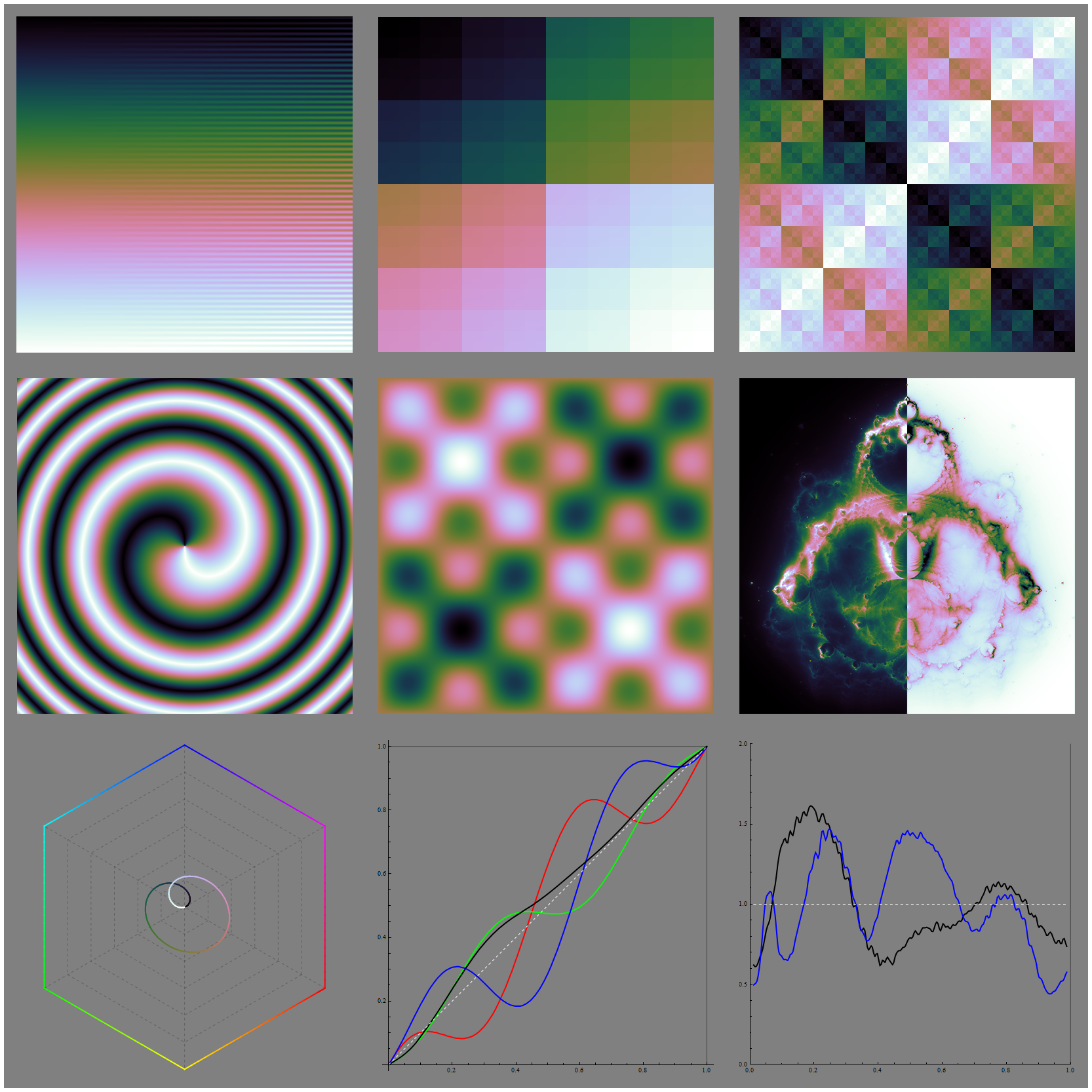
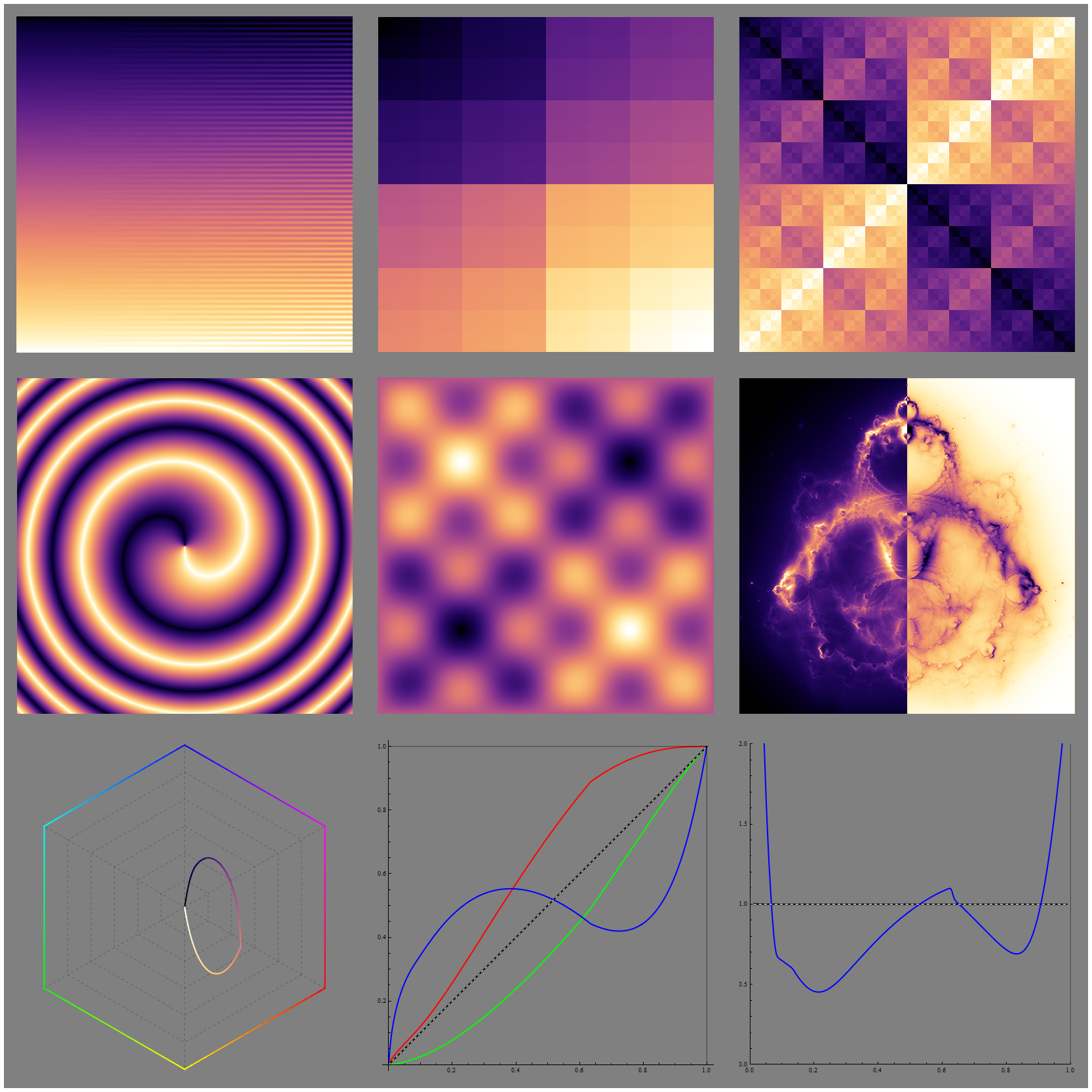
Not completely satisfied with any of the options mentioned so far, I decided to start from scratch. Issues exhibited by the Matplotlib colormaps made me question the utility of overly complicated color models, so I came up with a fairly simple approach. Start with a base colormap g(t) covering the desired hue range. Then mix g(t) with an appropriate amount of black or white so that the resulting color f(t) has lightness t (by "mix" I mean interpolate linearly in the RGB space). The exact proportion of black or white required to achieve the target lightness can be calculated by a numeric optimization algorithm such as bisection.
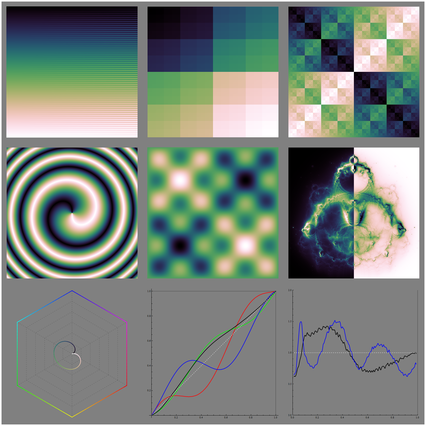
Resulting colormaps satisfy the lightness range and uniformity criteria by construction. Avoiding banding and ugly transitions proved to be the most significant obstacle. To construct the base maps, I employed smooth curves in the RGB space (piecewise-linear curves almost inevitably led to banding). The first two designs, [Hesperia] and [Lacerta], use Bezier curves with control points having HSV coordinates
| Hesperia | (250°, 1, 1), (330°, 2/3, 1), (50°, 1, 1) |
| Lacerta | (255°, 1, 1), (150°, 1, 1), (45°, 1, 1) |
Since of all the "rainbow" HSV(x, 1, 1) colors blue is the darkest and yellow is the lightest, the blue-yellow direction is naturally chromatically pure. Also, if we look at the constant L Lab slices, colors having the most chroma at low and high lightness are blue and yellow. However, I had to slightly tweak the hues to avoid resolution and smoothness issues.
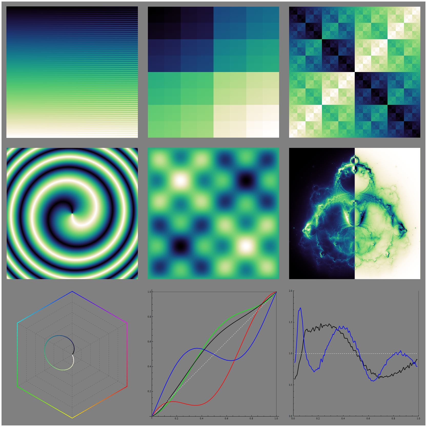
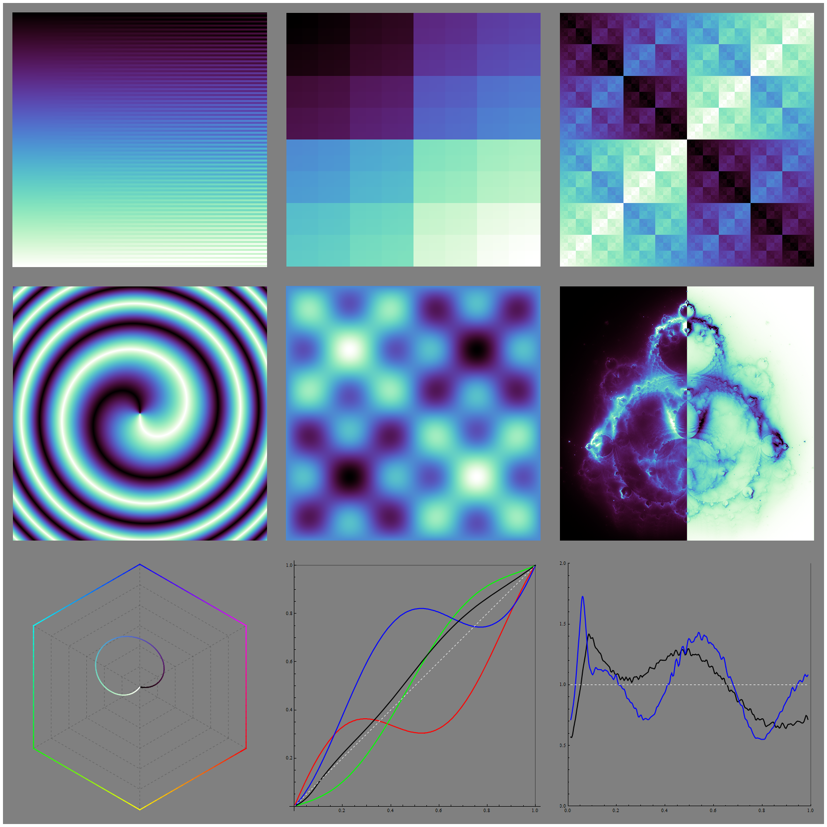
The third design, [Laguna], uses a circle lying in the R + G + B = 3/2 plane with the center at RGB(1/2, 1/2, 1/2) for the base colormap. The arc has a radius of 1/√6 and goes from magenta to green. The proposed colormaps mostly satisfy all of my criteria, but there is still much room for improvement. In particular, I fear that Hesperia's red-yellow region appears overly bright (Helmholtz–Kohlrausch effect?).
The lightness adjustment by black/white mixing process can also be applied to the existing colormaps, although it is not its intended use. The best example of such a hybrid is the [Modified Plasma].
List of all tested colormaps
Download all colormap data (CSV format with comments) as a single archive


Statistics
- Min L: minimal lightness
- Max L: maximal lightness
- L range: Max L - Min L
- Min L': minimal lightness derivative
- CV L': coefficient of variation (SD / Mean) of the lightness derivative
- Min |f'|: minimal norm of the Lab derivative
- CV |f'|: coefficient of variation (SD / Mean) of the norm of the Lab derivative
- Hue range: range of the angles spanned by the colormap projected along the RGB cube diagonal
- Chroma length: length of the colormap projection along the Lab L axis
- Chroma integral: ∫ |chroma| |dφ|, where φ is the chroma angle
- Mean |chroma|: mean length of the (a, b) vector in Lab colorspace
- Mean purity: mean of Max(r, g, b) - Min(r, g, b), indicates how close is the colormap to the pure HSV(x, 1, 1) colors
- Smooth: subjective smoothness assessment
| Name | Min L | Max L | L range | Min L' | CV L' | Min |f'| | CV |f'| | Hue range, ° | Chroma length | Chroma integral | Mean chroma | Mean purity | Smooth |
|---|---|---|---|---|---|---|---|---|---|---|---|---|---|
| RGB gray | 0 | 1 | 1 | 0.699 | 0.123 | 0.699 | 0.123 | 0 | 0 | 0 | 0 | 0 | + |
| L-Uniform gray | 0 | 1 | 1 | 1 | 0 | 1 | 0 | 0 | 0 | 0 | 0 | 0 | + |
| HSV Rainbow | 0.322 | 0.971 | 0.648 | -2.617 | 7.443 | 0.281 | 0.470 | 238 | 4.349 | 3.459 | 0.924 | 1 | − |
| CubeYF | 0.300 | 0.888 | 0.588 | 0.140 | 0.400 | 0.752 | 0.436 | 221 | 2.644 | 1.960 | 0.710 | 0.577 | + |
| Lin. L Rainbow | 0.010 | 1 | 0.990 | 0.255 | 0.092 | 0.990 | 0.523 | 289 | 3.404 | 1.966 | 0.449 | 0.405 | − |
| Cubehelix def. | 0 | 1 | 1 | 0.611 | 0.276 | 1.285 | 0.293 | 540 | 2.707 | 2.228 | 0.253 | 0.209 | + |
| Cubehelix +hue | 0 | 1 | 1 | 0.351 | 0.394 | 1.628 | 0.322 | 541 | 3.872 | 3.130 | 0.360 | 0.311 | − |
| Cubehelix Alt 1 | 0 | 1 | 1 | 0.620 | 0.250 | 1.382 | 0.253 | 360 | 1.962 | 1.456 | 0.247 | 0.209 | + |
| Cubehelix Alt 2 | 0 | 1 | 1 | 0.620 | 0.214 | 1.072 | 0.267 | 360 | 1.952 | 1.420 | 0.257 | 0.208 | + |
| Cubehelix Alt 3 | 0 | 1 | 1 | 0.590 | 0.311 | 1.354 | 0.273 | 245 | 2.157 | 1.317 | 0.349 | 0.313 | + |
| Cubehelix Alt 4 | 0 | 1 | 1 | 0.567 | 0.229 | 1.339 | 0.262 | 243 | 2.206 | 1.394 | 0.363 | 0.314 | + |
| Magma | 0.001 | 0.979 | 0.977 | 0.298 | 0.168 | 1.224 | 0.270 | 178 | 2.174 | 1.531 | 0.499 | 0.414 | + |
| Inferno | 0.001 | 0.979 | 0.978 | 0.299 | 0.159 | 1.330 | 0.267 | 180 | 2.581 | 1.864 | 0.583 | 0.517 | + |
| Plasma | 0.154 | 0.944 | 0.789 | 0.656 | 0.140 | 1.046 | 0.295 | 178 | 2.104 | 1.885 | 0.734 | 0.634 | + |
| Viridis | 0.149 | 0.909 | 0.759 | 0.717 | 0.055 | 1.318 | 0.192 | 234 | 2.062 | 1.765 | 0.512 | 0.458 | + |
| Hesperia | 0 | 1 | 1 | 1 | 0 | 1.150 | 0.620 | 162 | 2.268 | 1.302 | 0.473 | 0.377 | + |
| Lacerta | 0 | 1 | 1 | 1 | 0 | 1.164 | 0.453 | 207 | 2.538 | 1.224 | 0.399 | 0.308 | + |
| Laguna | 0 | 1 | 1 | 1 | 0 | 1.375 | 0.299 | 179 | 2.092 | 1.173 | 0.380 | 0.345 | + |
| Mod. Plasma | 0 | 1 | 1 | 1 | 0 | 1.388 | 0.616 | 178 | 2.688 | 1.639 | 0.549 | 0.461 | + |
| LA Olive-Blue | 0.144 | 0.984 | 0.840 | 0.363 | 0.272 | 1.150 | 0.193 | 183 | 1.149 | 0.821 | 0.272 | 0.224 | + |
| Morgenstemning | 0 | 1 | 1 | 0.037 | 0.599 | 0.995 | 0.470 | 222 | 3.346 | 2.130 | 0.472 | 0.438 | − |
| Black Body | 0 | 1 | 1 | 0.977 | 0.017 | 1.604 | 0.462 | 56 | 2.357 | 0.861 | 0.527 | 0.518 | − |
| Ext. Black Body | 0 | 1 | 1 | 0.623 | 0.134 | 1.778 | 0.510 | 159 | 4.097 | 2.040 | 0.675 | 0.592 | − |
| Kovesi KRYW | 0.050 | 1 | 0.950 | 0.528 | 0.089 | 1.211 | 0.389 | 48 | 2.510 | 0.833 | 0.668 | 0.657 | + |
| Kovesi BGYW | 0.152 | 1 | 0.848 | 0.790 | 0.005 | 1.017 | 0.700 | 194 | 3.080 | 1.669 | 0.678 | 0.538 | + |
References
- Good Colour Maps: How to Design Them. Peter Kovesi, arxiv.org, 2015.
- Rainbow Color Map (Still) Considered Harmful. D. Borland, R. M. Taylor II, IEEE Computer Graphics and Applications, vol.27, no. 2, pp. 14-17, March/April 2007
- Rainbow Color Map Critiques: An Overview and Annotated Bibliography. S. Eddins, Mathworks Technical Articles and Newsletters, 2014. [PDF]
- Face-based Luminance Matching for Perceptual Colormap Generation. G. Kindlmann, E. Reinhard, S. Creem, IEEE – Proceedings of the conference on Visualization ’02, 2002.
- A colour scheme for the display of astronomical intensity images. D. A. Green, Bulletin of the Astronomical Society of India, 39, pp. 289-295, 2011.
- Dimensions of color harmony. D. J. Polzella, D. A. Montgomery, Bulletin of the Psychonomic Society, Volume 31, Issue 5, pp 423–425, 1993.
- How to display data by color schemes compatible with red-green color perception deficiencies. M. Geissbuehler and T. Lasser, Opt. Express 21, 9862-9874 (2013)