Abstract
This page summarizes the research conducted during the development of Ascension's genetic algorithm and also serves as the user's guide. The genetic algorithm is briefly introduced and the problem of premature convergence is outlined. Many existing and novel techniques are then examined and the results of a large-scale experimental study are presented.
Contents
IntroductionThe role of diversity
Examined techniques
Experimental setup
Experimental results
Conclusion
References
API
Introduction
A genetic algorithm is inspired by the process of evolution. It maintains a population of solutions and relies on the principles of heredity, genetic variability and natural selection to improve the solutions over time. New solutions are created by means of sexual reproduction and replace the existing ones. There are two principal forms of GA:
- Generational: single algorithm iteration represents a single generation. Multiple solutions are created by means of reproduction and a large fraction of the population can be replaced.
- Steady-state: single algorithm iteration represents a single reproduction. Only one new solution is created, and only one solution may normally be replaced.
- Crossover: A new solution is created from the two parents by combining their elements.
- Mutation: Random changes are applied to the result.
Ascension employs the steady-state version, as it is far more flexible. It is especially good for experimentation, as various parts of can be modified independently without having to rewrite the whole algorithm. A steady-state iteration consists of the following steps:
- Selection: select two individuals from the population.
- Reproduction: create a new solution by performing a crossover between the selected solutions and then applying the mutation operator.
- Replacement: select a solution to be replaced by the newly created one and decide whether to actually perform the replacement.
- Select two distinct solutions at random.
- Create the child via crossover and mutation.
- Pick the worst parent for replacement.
- Accept the child only if it is better than the solution picked for replacement (elitist acceptance).
The role of diversity
Most basic GA examples found in textbooks and tutorials use selection and replacement strategies that ensure the reproduction and survival of the fittest solutions alone. This strategy may seem natural, but in the long term leads to poor performance. Good solutions proliferate exponentially, quickly taking over the entire population. The algorithm has no time for exploration, converging to a single local optimum early on. Maintaining a diverse population is therefore vital for solving complex multimodal problems. Diversity is a precious resource that should not be squandered. But simply maintaining it is not sufficient. It acts as a potential energy and must be "converted" to good solutions.
It is quite easy to modify the GA in order to achieve a near-perfect diversity preservation. But strategies that focus on diversity alone also tend to perform poorly, as they sacrifice depth for breadth. It appears that a god GA variant must satisfy contradictory requirements. The observation that such contradictions arise in many engeneering problems lies at the heart of TRIZ (ТРИЗ, Теория Решения Изобретательских Задач, Theory of Inventive Problem Solving). Although TRIZ was developed for engineering problems specifically, its key idea is very much relevant to the design of efficient metaheuristics: an inventive solution does not compromise the conflicting objectives, but resolves the contradiction dialectically, on a deeper level. Simulated annealing is a great example of an inventive solution: instead of relying on a fixed exploration-exploitation tradeoff, it achieves the conflicting objectives by gradually changing the nature of the search. Tabu search also benefits from this strategy.
TRIZ sheds a new light upon the GA and allows to construct the diversity preservation methods in a systematic manner. A general principle that can be used to resolve the exploration-exploitation contradiction is the division of labor: divide the search into parts specializing in each objective. A variety of GA variants can be constructed by choosing different exploration methods, division types and part interactions. The division can be temporal, spatial or rank-based, further abbreviated as TD, SD and RD. Curiously, SD and TD types even have corresponding TRIZ principles: "3. Local quality" and "15. Dynamics".
Examined techniques
The behavior of many GA variants can be analysed using a very simple model. Suppose that the population consists of two solution types, A and B, B being the better one. Crossover produces an offspring having the type of a random parent and mutation does nothing. This model represents a problem with two local optima and a mutation that can only make small changes, but cannot change the solution's basin of attraction. An important quantity in this model is the takeover time - the mean time until a single type B solution takes over the entire population. Takeover time quantifies GA's exploration ability. Approximate solutions to this model were be obtained by ignoring the finite population size effects (genetic drift), which led to differential equations describing the GA dynamics. Due to the nature of such approximation, the takeover time was defined as the time between B(t) = 1 and A(t) = 1.
| Definitions | |
| N | Population Size |
| A | Number of solutions of type A |
| B | Number of solutions of type B |
| ΔB | Expected change of B after a single steady state iteration |
| α | A / N |
| β | B / N |
| τ | Takeover time in generations |
| r | Normalized rank, 0 corresponding to the best and 1 to the worst solution. |
| t | Normalized time, 0 corresponding to the start of the algorithm and 1 to the maximum number of fitness function evaluations being reached. |
| P | A selection or replacement parameter |
Score-based replacement
Worst in population
ΔB = β, τ = Ln NWorst parent
ΔB = α β, τ = 2 Ln N
This method can be considered a weak form of diversity maintenance, since the child is likely to be similar to at least one of the parents.Random parent
ΔB = α β / 2, τ = 4 Ln NInverse rank-proportional: pick an individual at random with probability proportional to r-P.
Score-based selection
Fitness-proportional: select each parent with probability proportional to fitness. This popular method was not implemented as it is not invariant under linear fitness transformations. This means that the raw score values would have to be rescaled first, which would complicate either the algorithm or the user's life. Moreover, if the worst parent is picked for replacement and the acceptance is elitist, fitness-proportional selection is unnecessary because there is already enough evolutionary pressure.
Rank-proportional: select each parent with probability proportional to (1 - r)P, P > 0, r-P, P < 0. For integer values of P, equivalent to selecting |P| + 1 individuals at random and then selecting the best (P > 0) or the worst (P < 0). This selection method entirely sidesteps fitness scaling issues. For the reasons already outlined, positive values of P are not really necessary. If P > 0, the takeover time actually exceeds thats of P = 0, since the chance of selecting an A-B pair becomes exceedingly low with time. Nonetheless, it would be fair to classify this setting as a quickly converging one, as the initial growth of high-fitness solutions is more rapid, and the remaining lower fitness solutions are rarely selected.
Inverse rank-proportional selection (P < 0) may seem counterintuitive, but can be advantageous. Even for P = -1, the takeover time is very long. It would take on average about N generations till an A-B pair is selected from the initial population. This results in a steadier process: if a very good solution is discovered, it is effectively set aside until the rest of the population catches up. Fitness is also correlated with the distance to the best solution in the population, so this setting indirectly favors unique solutions.
Fitness-uniform selection
ΔB = 1 / 2, τ = 2
Select a fitness value uniformly at random from the range of values in the population, then select an individual with the closest fitness. Introduced in [1] as a way to preserve diversity. However, has an opposite effect when applied to the baseline steady-state GA. Demonstrated poor results during preliminary testing and was excluded from further experiments.Near rank selection
ΔB = 1 / N, τ = N
Select an integer k uniformly at random from the interval [0 .. N - 2], return the individuals with ranks k, k + 1. The idea behind this method is that the ranking implicitly defines a kind of niching. Nearby rank selection ensures that such niches can coexist for long periods of time.
Distance-based selection
Distance-based techniques rely on a distance operator that quantifies the degree of dissimilarity between two solutions. In fact it only needs to satisfy two of the three properties of a true distance - identity and symmetry, but not necessarily the triangle inequality. Calculating the distance can be as expensive as evaluating the fitness function. For this reason, many well known techniques such as niching and clearing that require many distance calculations were not implemented.
Pair distance. Select |P| distinct individuals at random, pick the pair with the maximal (P > 0) or the minimal (P < 0) distance. Arguments in favour of both positive and negative distance-based selection can be made. On the one hand, positive selection increases the variativity of the offspring, which should be good for diversity. On the other hand, in many problems dissimilar parents are unlikely to produce a good offspring. Negative distance selection can therefore be beneficial, mimicking speciation. Authors of NEAT used explicit speciation for this reason [2].
Distance to best. Select |P| distinct individuals at random, pick two solutions with the maximal (P > 0) or the minimal (P < 0) distance to the best in population.
Distance-based replacement
A child's contribution to diversity (henceforth called originality) can be measured in two different ways: by its distance to either the most similar parent or to the best individual in population. All presented distance-based replacement methods support both.
Least original parent. Pick the most similar or the central parent depending on the originality measure. This options excels at preserving diversity, but results in very slow convergence.
τ = ∞Novelty. Pick the worst parent if its replacement would increase the distance to the other parent or to the best in population depending on originality measure, otherwise pick the least original parent. Effectively a slightly less strict version of the least original parent replacement.
τ = ∞Least original worse parent. If the child is better than both parents, pick the least original one, otherwise the worst one. The logic behind this method is that in such a fortunate case, we can preserve the diversity and still gain in terms of fitness. In effect, the least original parent that is worse than the child will be replaced assuming elitist acceptance.
Compound hard RD. Use thre least original parent replacement if the child is better than the population median, otherwise use the worst parent replacement. The idea behind this method is to prevent the best solutions from quickly taking over the population.
Compound hard SD. Partition the population in two sections. Use the worst parent replacement if both parents come from the first section, otherwise use use the least original parent replacement.
Compound hard TD. If t < 1 - 1 / P, use the least original parent replacement, else if t < 1 - 1 / P2, use the worst parent replacement, else pick the worst individual in population. Assuming that the first stage should take more time than the last two combined due to slower convergence, we arrive at a guesstimate P = 3 which minimizes the worst case relative error (all stages take at least 2 / 3 of their optimal time). This value was used in all the experiments.
It is possible to transition between exploration and exploitation smoothly. Suppose that the probability of using an exploitation strategy is given by tq. Then the effective exploitation time is ∫tq dt = 1 / (1 + q). The number of exploitation events per generation follows a binomial distribution with mean N tq. Near t = 0 it can be approximated by a Poisson distribution, which gives the probability of an exploitation-free generation Exp(-N tq). The effective exploration time can then be defined as ∫ Exp(-N tq) dt ≈ t-1 / q ((1 / q)!) ≈ t-1 / q. A good value of q can be obtained by maximizing the product of the exploration and exploitation times since both are important, which gives q ≈ Ln(N) + 1. This estimate is used many times in this work, except that for the rank-based methods the value of q is sometimes reduced by 1 since the worst parent replacement introduces an additional rank bias.
- Compound soft RD, TD. Use the worst parent replacement with probability xLn(N) + 1, otherwise use the least original parent replacement, where
- RD: x is the normalized rank of the solution with the score closest to thats of the child
- TD: x = t
Topological selection
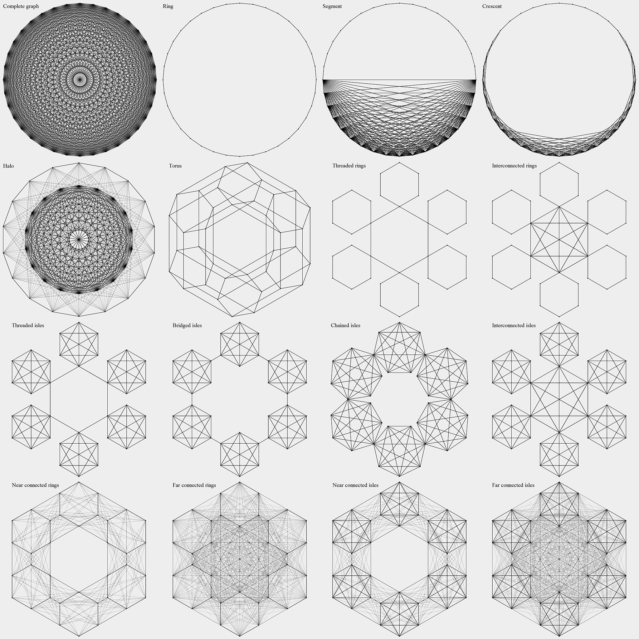
Methods from this group impose a certain structure upon the population in order to increase the takeover time. This structure (topology) is defined by a graph whose vertices correspond to the individuals. Selection is performed by picking a random vertex and then picking a random edge originating from that vertex. The graph can be weighted, in which case the edge selection probabilities are proportional to their weights. Cellular genetic algorithms [3] belong to this category, with graph being a regular grid. Calculating the takeover times is generally hard, but they can be bounded by the graph diameter. Asymptotics marked with "?" are educated guesses. All the topologies under consideration have a well-defined structure, which makes the explicit graph representation unnecessary. Instead, the selection process can be defined in terms of vertex indices ranging from 0 to N - 1.
Ring. Each vertex is connected to two neighbours (i + 1) mod N, (i - 1) mod N. The slowest of the examined topologies. τ = O(N)
Leaky ring. An attempt to accelerate the ring topology by adding weak edges between the distant vertices: there is a small chance (1 / N) to select a random vertex distinct from i instead of a neighbour. One far edge is selected per generation on average. τ = O(N)?
Leaky ring TD. Same as leaky ring, but the probability of a far edge is given by tLn(N) + 1.
Torus. Each vertex is connected to four neighbours on a square grid wrapping around the edges. τ = O(√N).
Segment. A complete graph (N / 2 vertices) and a path graph (N / 2 vertices) connecting its two vertices. τ = O(N).
Segment TD. Same as segment, but the path graph / complete grap vertex ratio varies linearly from 1 to 0 with time.
Crescent. Graph connectivity varies in space. Vertices i and j are connected if and only if d(i, j, N) < Min(R(i, N), R(j, N)), where d(i, j, N) = Min(|i - j|, N - |i - j|) is the modulo distance and R(i, N) = N / 22 Min(i, N - i) / N. In effect, the graph smoothly transitions from a linear to a fully connected topology.
Variable degree TD. Graph connectivity varies with time. The index of the first vertex is selected at random, the index of the second vertex is obtained by adding a random offset from 1 to Floor((N - 1)t) and taking the result modulo N.
Halo. The population is divided into two parts, a ring and a complete graph both of size N / 2. A vertex is selected at random, and if it belongs to the ring, there is a chance (2 / N) of the second vertex being selected from the other part instead of selecting a natural neighbor. τ = O(N)?
Directed halo. Preliminary convergence can also be prevented by restricting the flow of information to one direction. This topology also consists of a ring and a complete graph both of size N / 2. A vertex pair is selected either from one of the parts, or from both parts at random, with each option having the probability 1 / 3. In the latter case, the parent belonging to the complete graph is selected for replacement, which prevents the pollution of the ring. Otherwise the worst parent is replaced. This is the only method in this section that relies on a specific replacement (Ascension option "Digraph"). τ = O(N).
Another popular group of techniques also topological in nature are the island genetic algorithms [4]. The population is partitioned into a number of weakly interacting subpopulations ("islands"), which increases the takeover time. The traditional island interaction method is the exchange of the individuals from different islands at regular time intervals ("migration"). Ascension features a number of island-like methods with island interactions being defined implicitly, through the population topology alone. The subpopulations can have a ring or a complete graph topology, called simply "isles" in the latter case. The connections between them can also form a ring or a complete graph, with several options in case of a ring:
- Threading: subpopulations connected by a ring going through a single vertex of each one
- Bridging: nearby subpopulations connected by a bridging edge
- Chaining: nearby subpopulations joined via common vertex
- Interconnection: subpopulations connected by a complete graph that includes a single vertex from each one
This results in eight possible topologies. Two of them (bridged rings and chained rings) are not sufficiently distinct from the ring topology (effectively two rings intertwined, τ = O(N)) and thus were not implemented. The number of subpopulations was set to √N in all cases (N assumed to be a square), a middle ground most distinct from both extremes. This choice also makes the island topologies directly comparable to the torus, which can be viewed as √N linked subpopulations.
- Threaded rings. τ = O(√N).
- Interconnected rings. τ = O(√N).
- Threaded isles. An interesting case, since the graph diameter (O(√N)) seems to differ greatly from the takeover time. There are √N thread edges with selection probability 2 / √N, so τ = O(N)?
- Bridged isles. Takeover dynamics similar to thats of threaded isles. τ = O(N)?
- Chained isles. τ = O(√N Ln N)?
- Interconnected isles. τ = O(Ln N)?
Another way to create an island structure is to have a small chance of randomly selecting the parents from distinct subpopulations. This probability was set to 1 / √N so that there is one such event per subpopulation per generation on average. The subpopulations can be selected at random or form a ring. Combined with two possible topologies of the subpopulations themselves, this gives four more options:
- Random near connected rings. τ = O(√N).
- Random far connected rings. τ = O(√N)?
- Random near connected isles. τ = O(√N Ln N)?
- Random far connected isles. τ = O(Ln(N)2)?
Injection of new solutions
Injection of new solutions into the population can serve two purposes: it provides new genetic material and it creates fitness "holes" that can then be occupied by offspring less fit than the rest of the population.
- Rare influx. Pick the worst parent for replacement. If the child is better than both parents, replace the other parent with a new solution. Such occurences are generally very rare.
- Influx RD, SD, TD. With probability xq create the child from scratch instead of using the normal reproduction and replace the worst parent unconditionally, otherwise pick the worst parent for replacement.
- RD: x is the normalized rank of the worst parent, q = Ln(N).
- SD: x is the normalized index of the worst parent, q = Ln(N) + 1.
- TD: x = 1 - t, q = Ln(N) + 1.
Non-elitist acceptance
Techniques from this category may accept the child even if it is worse than the solution being replaced, which should prevent the population from getting stuck in a local optimum.
- Unconditional. Accept the child regardless of its fitness. Although this methods accepts lots of very bad solutions, it can be viable in principle if used with the worst parent replacement, since that would guarantee that the best solution in the population can never be replaced.
- Unconditional with inverse rank TD replacement. Select the solution for replacement with probability rp(t), where p(t) interpolates between p(0) = 1, p(1 / 2) = Ln(N) + 1, p(1) = N, accept the child unconditionally. The idea is to achieve an annealing-like effect, starting with an almost random search and finishing with a greedy one by controlling which solutions are replaced.
Hybridization with simulated annealing has been reported in the literature. However, this approach requires at least two extra parameters, the initial and the final annealing temperatures. The former can be automatically selected before running the algorithm, but the latter can't. It is possible to achieve a similar effect without the additional parameters by using the quantiles of the population fitness as the acceptance threshold:
- Threshold. Accept the child if it is better than the population median.
- Threshold SD. Accept the child if it is better than the solution with rank equal to the index of the replaced solution.
- Threshold TD. Accept the child if it is better than the solution with rank N (1 - t).
Another possibility is to take the originality into acount:
- Originality RD, SD, TD. Accept the child if it is better than the solution being replaced, otherwise accept it if it increases the originality with probability xq.
- RD: x is the normalized rank of the solution being replaced, q = Ln(N).
- SD: x is the normalized index of the solution being replaced, q = Ln(N) + 1.
- TD: x = 1 - t, q = Ln(N) + 1.
Experimental setup
Comparing multiple GA configurations is not a trivial task. It is quite easy to outperform a baseline GA if the population size is kept constant across the tests. Such a comparison would have been flawed, as the diversity deficit of the faster converging configurations could be compensated by increasing the population size. Given a fixed computational budget, each configuration has its own optimal population size, the less the better its diversity preservation is. Thompson sampling was therefore employed to select the optimal value in each case without a huge computational cost. The tested values are a subset of squares (for topological selection compatibility), with the ratio of two subsequent values never exceeding 4 / 3: 4, 9, 16, 25, 36, 49, 64, 81, 100, 121, 144, 169, 225, 289, 361, 441, 576, 729, 961, 1225, 1600, 2116, 2809, 3721, 4900, 6400, 8464. Each configuration was normally tested until the sample size reached 1000, although the underperforming ones were shut down earlier. A number of multimodal problems that could in principle benefit from diversity preservation was selected for testing.
Optima grid
A 2D test function similar to Rastrigin's. Consists of a square grid of local optima plus the global quadratic term.
cx = Cos(τ F x)
cy = Cos(τ F y)
f(x, y) = x2 + y2 + √3 - cx - cy - cx cy
- NFE = 262144
- F = 20
- Domain: [-1 .. 1]2
- Minimum: f(0, 0) = 0
- Crossover: one coordinate taken from each parent
- Mutation: (x', y') = (x, y) + U (Cos(θ), Sin(θ)) / (2 F), where x', y' are the new coordinates, θ is a random angle and U is a uniform random variable on the unit interval. This mutation was designed specifically for testing. It introduces small changes but unable to jump between different local optima.
- Distance: Euclidean
Despite being multimodal, this function does not benefit from diversity preservation. Separability is likely the reason: the global minimum can be found by optimizing it along the x and y axes independently, which greatly simplifies the optimization.
Rotated optima grid
Same as the optima grid, but the coordinates are first rotated by the arctangent of the golden ratio. This transformation destroys the separability and makes this function much more difficult.
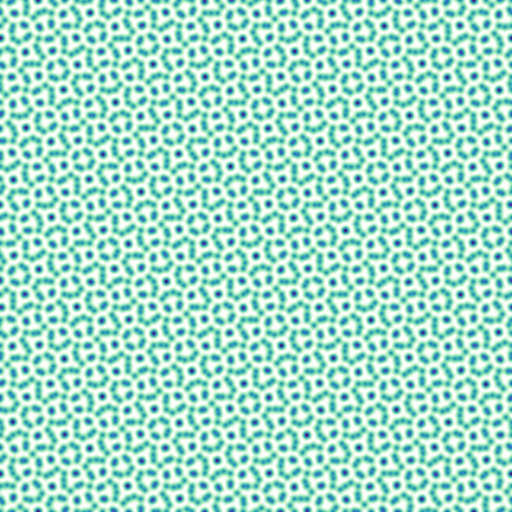
Double optima grid
A sum of two optima grids, one rotated by the arctangent of the golden ratio and the other unrotated. Combined with the lack of the global term, this resuts in a complicated moire-like pattern. Parameters identical to the previous two problems.
Fractal
A 2D fractal lanscape given by the superposition of rotated cosine waves with exponentially increasing frequencies and exponentially decaying amplitudes:
f(x, y) = ( (kA - 1) / kA ) ∑i kA-i ( 1 - Cos( τ kFi ( x Cos(i θ) + y Sin(i θ) ) ) ),
where θ equals τ divided by the golden ratio and i varies from 0 to ∞.
- NFE = 262144
- kF = 2, kA = 21 / 4, fractal dimension = 2.75
- Domain: [-0.5 .. 2.5]2
- Minimum: f(0, 0) = 0
- Crossover: extended line. The child is the result of a linear blending between the parents: (x, y) = α (x, y)A + (1 - α) (x, y)B. α comes from a distribution uniform on the [0 .. 1] interval and having two exponentially decaying tails attached at α < 0 and α > 1 with 1 / e decay length 1 / 4.
- Mutation: none
- Distance: Euclidean
The fractal nature of the landscape results in a challenging test function. The difficulty can be controlled by adjusting the fractal dimension. The domain was intentionally shifted to avoid the global optimum being located in the center. This was done to negate the effect of any potential bias of the crossover towards the center.

Funnel
An important feature of many real problems is the so called globally convex (also called funnel or big valley) fitness landscape: a multitude of local optimal, with the global one located in the "center" (the distance to the global optimum is negatively correlated with the quality of the local optima). This test function was designed to imitate such structure. It is the sum of multiple 1D functions with two local optima:
f(x) = ∑ √1 - (2 | |xi| - 1 / 2|)2 + |xi| / n,
where n is the problem size.
- NFE = 262144
- Problem size: 16
- Domain: [-1 .. 1]
- Minimum: xi = 0, f(x) = 0
- Crossover: discrete uniform
- Mutation: A random offset of the form ±U2 / 2 is added to xi with probability 1 / 16, where U is a uniform random number on the unit interval. The result is then cyclically wrapped into [-1 .. 1] interval.
- Distance: sum of cyclic distances, ∑ |Min(|xi - yi|, 2 - |xi - yi|)|
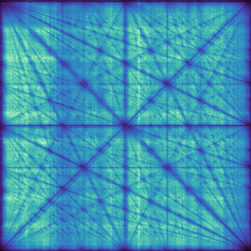
CoreWar
CoreWar is a programming game in which programs written in assembly-like language fight each other in virtual memory. Each program has a number of integer parameters that must be optimized for best combat efficiency. Due to complex parameter interactions this is usually a difficult problem. This test relies on a precalculated 800 x 800 score surface to avoid the computational cost of emulating the battles. The most challenging surface was chosen from several instances. One instance that had very little parameter interactions was found to be particularly easy. This is further evidence of separability being a good difficulty indicator.
- NFE = 16384
- Crossover: one parameter taken from each parent
- Mutation: A log-uniform offset is added to each parameter with probability 1 / 2. The result is taken modulo 800.
- Distance: Sum of logarithms of parameter modulo distances incremented by 1.
Heilbronn
The problem consists of placing a number of points within a given 2D region so as to maximize the area of the minimal triangle formed by any three points. This problem quickly becomes very difficult as the number of points increases. An anomalous case, with most configurations failing and unconditional acceptance performing the best.
- NFE = 65536
- Number of points: 10
- Region: unit square
- Maximum: 0.0465+
- Crossover: The child is constructed from the parent points, selecting the best point at each step and alternating the parents.
- Mutation: An offset with a random angle and log-uniform distributed radius is added to a random point.
- Distance: Sum of the minimal distances of each point of each solution to any other point of the other solution.
Binary epistasis
Consider the simplest binary minimization problem with interacting variables: f(0, 0) = 0, f(1, 1) = 1, f(0, 1) = f(1, 0) = 2. A more difficult problem can be constructed by concatenating multiple 2-bit blocks and taking the sum of f over them. If the population has converged to the wrong local optimum on a certain block, it would take a long time (quadratic in problem size) for it to get out by a lucky mutation. This is the only test which does not use a fixed computational budget. Instead, the algorithm was executed until the global optimum was found and the NFE was recorded.
- Problem size: 256 bits
- Minimum: 0
- Mutation: each bit inverted with probability 2 / 256
- Crossover: single point. Chosen intentionally, as it makes the problem more difficult due to lower child variability.
Hierarchy
A hierarchic version of the binary epistasis, subject to maximization. The score is calculated by going through consecutive 2-bit blocks and adding S0 in case of 00 and S1 in case of 11. The bit string is then downsampled by replacing 00 with 0, 11 with 1 and the other blocks with any other symbol. Block score values are then multiplied by K and exchanged. The process is repeated until there is only one bit left. K factor ensures that the higher levels have the most impact. Alternation of the block scores makes the problem deceptive: bits optimal at one level are suboptimal at the next one. The impact of diversity preservation on this problem was particularly large.
- Problem size: 256 bits
- S0 = 1, S1 = 2, K = 4
- Maximum: 43520
- Mutation: each bit inverted with probability 3 / 256
- Crossover: two point
Minimal linear arrangement
The problem consists of arranging the integers from 1 to n2 on a n by n grid so as to minimize the sum of the absolute differences between the numbers in adjacent squares. The optimal values are given by A195647.
- Problem size: 8 x 8
- Minumum: 472
- Mutation: subtour reversal
- Crossover: partially matched
Experimental Results
The results are presented in the form of effect sizes. Specifically, Glass's Δ was used: Δ = ±(μx - μc) / σc, where μx is the mean result of an experimental configuration and μc and σc are the mean and the standard deviation of the baseline algorithm's results. The sign was chosen for each problem so that the positive values correspond to better results. This measure was chosen as it preserves the ranking of the algorithms by mean. In the context of the current study, an effect size of 1 should be considered very large. Suppose that the baseline results are exponentially distributed starting at the global optimum. Then the oracle algorithm always finding this optimum would have Δ = 1. Positive effect sizes with p-values less than 0.01 are highlighted. "S", "R", "A" and "O" prefixes stand for selection, replacement, acceptance and originality. "RPS" stands relative population size and is calculated as the geometric mean of the ratio of the optimal population size of an experimental configuration to thats of the baseline algorithm.
Rating measures an overall performance across all problems calculated using an Elo-type system. The score of one configuration against another on a particular problem is defined as the probability of it achieving a better result in a single run. Normal approximation was used: S(A, B) = NCDF(±(μA - μB) / √σA2 + σB2), where NCDF is the cumulative distribution function of the standard normal distribution. In the Elo model, the expected score is given by the logistic function: ES(A, B) = 1 / (1 + Exp(RB - RA)), where RA and RB are the configuration ratings. The ratings were initialized with zeroes and then iteratively updated using an inverse logistic function: R = Rμ + Ln(Sμ / (1 - Sμ)), whre Sμ is the mean score against other configurations across all problems and Rμ is their mean rating. The results were then normalized by substracting the rating of the baseline configuration.
| Configuration | Grid | RotGrid | DoubleGrid | Fractal | Funnel | ScoreSurf | Heilbronn | MinLA | Hierarchy | BinEpistasis | Minimum | Rating | RPS |
|---|---|---|---|---|---|---|---|---|---|---|---|---|---|
| R.WorstParent | 0.00 | 0.00 | 0.00 | 0.00 | 0.00 | 0.00 | 0.00 | 0.00 | 0.00 | 0.00 | 0.00 | 0.00 | 1.00 |
| R.Worst | -0.03 | -0.07 | -0.06 | -0.87 | -0.19 | -0.01 | -0.17 | 0.00 | 0.24 | -0.01 | -0.87 | -0.14 | 2.64 |
| R.RandParent | -0.17 | -0.21 | 0.06 | -0.01 | -0.18 | 0.06 | -0.13 | 0.09 | 0.40 | 0.32 | -0.21 | 0.01 | 0.65 |
| R.InvRank1 | -0.18 | -0.12 | -0.14 | -0.83 | -0.44 | -0.01 | -0.22 | -0.07 | -0.16 | -0.33 | -0.83 | -0.25 | 2.36 |
| S.Ring | -1.08 | 0.55 | 1.73 | -1.40 | 0.70 | 1.68 | -0.50 | 0.40 | 1.68 | -0.24 | -1.40 | 0.28 | 0.60 |
| S.Torus | -0.18 | 0.56 | 1.85 | -0.25 | 0.57 | 1.04 | -0.23 | 0.22 | 1.58 | 0.65 | -0.25 | 0.52 | 0.91 |
| S.LeakyRing | -0.78 | 0.55 | 1.75 | -1.46 | 0.66 | 1.67 | -0.43 | 0.37 | 1.58 | 0.22 | -1.46 | 0.32 | 0.67 |
| S.LeakyRingTD | -0.55 | 0.45 | 1.70 | -1.42 | 0.84 | 1.54 | -0.55 | 0.52 | 4.01 | -- | -1.42 | 0.47 | 0.62 |
| S.Segment | -0.53 | 0.37 | 1.18 | -0.23 | 0.46 | 1.05 | -0.30 | 0.29 | 0.67 | -1.10 | -1.10 | 0.21 | 0.71 |
| S.SegmentTD | -0.21 | 0.14 | 1.13 | -0.72 | 0.84 | 1.04 | -0.74 | 0.44 | 2.04 | -- | -0.74 | 0.35 | 0.50 |
| S.Crescent | -0.38 | 0.40 | 1.12 | 0.09 | 0.46 | 0.85 | -0.24 | 0.18 | 0.69 | -1.01 | -1.01 | 0.23 | 0.87 |
| S.VarDegreeTD | -0.10 | -0.01 | 1.02 | -0.68 | 0.90 | 0.81 | -0.75 | 0.42 | 3.96 | -- | -0.75 | 0.39 | 0.48 |
| S.Halo | -0.50 | 0.36 | 1.25 | -0.21 | -0.30 | 1.02 | -0.26 | 0.30 | 0.07 | -2.12 | -2.12 | 0.05 | 0.74 |
| S.DirHalo | -0.40 | -0.08 | 0.93 | -0.19 | 0.02 | 0.75 | -0.53 | 0.27 | 1.86 | -1.09 | -1.09 | 0.10 | 0.54 |
| S.RandNearConRings | -0.43 | 0.61 | 1.84 | -0.98 | 0.59 | 1.46 | -0.32 | 0.33 | 1.34 | 0.36 | -0.98 | 0.41 | 0.67 |
| S.RandFarConRings | -0.20 | 0.64 | 1.85 | -0.92 | 0.46 | 1.47 | -0.21 | 0.21 | 0.63 | 0.39 | -0.92 | 0.38 | 0.67 |
| S.RandNearConIsles | -0.50 | 0.50 | 1.38 | 0.91 | 0.57 | 0.78 | -0.25 | 0.37 | 1.75 | 0.34 | -0.50 | 0.51 | 0.95 |
| S.RandFarConIsles | -0.23 | 0.51 | 1.28 | 0.86 | 0.39 | 0.75 | -0.20 | 0.26 | 0.92 | 0.43 | -0.23 | 0.45 | 1.01 |
| S.ThreadedRings | -0.76 | 0.56 | 1.74 | -1.30 | 0.26 | 1.62 | -0.40 | 0.30 | 0.52 | -0.87 | -1.30 | 0.14 | 0.70 |
| S.InterconRings | -0.67 | 0.58 | 1.66 | -1.13 | -1.29 | 1.55 | -0.42 | 0.12 | -0.30 | -2.62 | -2.62 | -0.14 | 0.65 |
| S.ThreadedIsles | -1.13 | 0.47 | 1.33 | 1.00 | 0.53 | 1.04 | -0.41 | 0.49 | 1.16 | -0.86 | -1.13 | 0.36 | 0.78 |
| S.BridgedIsles | -1.18 | 0.45 | 1.34 | 0.98 | 0.59 | 1.03 | -0.40 | 0.51 | 1.18 | -0.81 | -1.18 | 0.36 | 0.81 |
| S.ChainedIsles | -0.54 | 0.48 | 1.32 | 0.95 | 0.58 | 0.80 | -0.29 | 0.30 | 1.60 | 0.21 | -0.54 | 0.47 | 0.85 |
| S.InterconIsles | -0.52 | 0.46 | 1.32 | 0.91 | 0.19 | 0.92 | -0.34 | 0.32 | 0.37 | -0.42 | -0.52 | 0.29 | 0.93 |
| S.DisconIslesTD | -0.23 | 0.10 | 0.89 | 0.55 | 0.81 | 0.50 | -0.80 | 0.66 | 3.45 | -- | -0.80 | 0.48 | 0.58 |
| S.RankProp1 | 0.05 | 0.15 | -0.08 | -0.18 | -0.22 | -0.01 | 0.09 | -0.00 | -0.23 | -0.66 | -0.66 | -0.09 | 1.74 |
| S.RankPropNeg1 | -0.21 | -0.61 | 0.26 | -0.81 | 0.03 | 0.04 | -0.37 | 0.13 | 3.21 | 1.01 | -0.81 | 0.09 | 0.60 |
| S.RankPropNeg2 | -0.32 | -0.84 | 0.37 | -1.31 | -0.07 | 0.04 | -0.64 | 0.10 | 3.00 | 0.93 | -1.31 | -0.04 | 0.52 |
| S.NearRank | -0.28 | -1.03 | -0.60 | -1.14 | -0.69 | 0.11 | -0.62 | 0.15 | 3.13 | 0.57 | -1.14 | -0.17 | 0.54 |
| S.Dist3 | -0.33 | -0.84 | -0.94 | -0.02 | 0.37 | -0.37 | 0.12 | 0.31 | 0.11 | 1.01 | -0.94 | -0.02 | 0.89 |
| S.DistNeg3 | -0.09 | 0.16 | 0.99 | 1.22 | -1.30 | 0.24 | 0.06 | -0.06 | -0.14 | -4.03 | -4.03 | -0.04 | 1.21 |
| S.DistToBest3 | -1.31 | -1.49 | -0.94 | -0.36 | 0.37 | -0.14 | -0.54 | 0.07 | 0.52 | 0.89 | -1.49 | -0.21 | 0.86 |
| R.InfluxRare | 0.02 | 0.11 | -0.04 | 0.21 | -0.79 | -0.02 | 0.31 | 0.20 | -0.12 | 0.57 | -0.79 | 0.04 | 0.54 |
| R.InfluxRD | -0.71 | -0.11 | -0.16 | -0.20 | -0.98 | -0.12 | -0.19 | -0.44 | -0.37 | -1.26 | -1.26 | -0.39 | 0.85 |
| R.InfluxSD | -1.04 | -0.48 | -0.26 | -0.31 | -1.05 | -0.17 | -0.28 | -0.48 | -0.40 | -1.23 | -1.23 | -0.49 | 0.76 |
| R.InfluxTD | -0.21 | 0.31 | -0.15 | -0.13 | -0.79 | -0.06 | 0.23 | -0.23 | -0.44 | -- | -0.79 | -0.14 | 0.92 |
| A.Threshold | -0.08 | -0.02 | -0.04 | -0.13 | -0.12 | -0.02 | 0.01 | 0.10 | -0.09 | -0.01 | -0.13 | -0.04 | 1.19 |
| A.ThresholdSD | -0.11 | -0.02 | -0.11 | -0.16 | -0.20 | -0.02 | 0.05 | 0.05 | -0.12 | -0.18 | -0.20 | -0.07 | 0.94 |
| A.ThresholdTD | -0.44 | 0.09 | -0.15 | -0.88 | -0.48 | -0.04 | 0.12 | 0.06 | -0.31 | -- | -0.88 | -0.22 | 1.42 |
| A.Uncond | -3.94 | 0.16 | -1.19 | -1.30 | -3.71 | -0.50 | 0.42 | -1.31 | -0.92 | -4.21 | -4.21 | -0.92 | 0.93 |
| A.DistToParentRD | -0.02 | 0.47 | -0.05 | -0.48 | -0.13 | -0.02 | 0.11 | -0.07 | -0.07 | -0.05 | -0.48 | -0.02 | 0.74 |
| A.DistToBestRD | -0.84 | -0.38 | -0.25 | -0.71 | -0.08 | -0.11 | 0.04 | -0.07 | -0.09 | -0.13 | -0.84 | -0.25 | 0.76 |
| A.DistToParentSD | -0.49 | -0.18 | -0.05 | -0.34 | -0.17 | -0.01 | 0.02 | -0.12 | -0.08 | -0.02 | -0.49 | -0.15 | 0.92 |
| A.DistToBestSD | -0.92 | -0.82 | -0.36 | -0.31 | -0.16 | -0.10 | -0.07 | -0.11 | -0.09 | -0.05 | -0.92 | -0.29 | 0.98 |
| A.DistToParentTD | 0.23 | 0.93 | -0.05 | -0.63 | 0.01 | -0.00 | 0.06 | 0.06 | -0.08 | -- | -0.63 | 0.08 | 0.70 |
| A.DistToBestTD | -1.68 | -0.50 | -0.36 | -0.60 | 0.04 | -0.22 | 0.06 | 0.19 | -0.05 | -- | -1.68 | -0.26 | 0.73 |
| R.InvRank6_UC | -1.05 | 0.05 | -0.38 | -1.01 | -0.52 | -0.07 | -0.09 | 0.06 | -0.20 | -0.36 | -1.05 | -0.36 | 1.87 |
| R.InvRankTD_UC | -0.61 | 0.51 | -0.37 | -1.25 | -0.98 | 0.29 | 0.13 | 0.16 | -0.41 | -- | -1.25 | -0.27 | 0.99 |
| R.SimParent | -0.54 | -0.77 | 0.16 | -1.97 | -0.00 | 0.38 | -0.97 | -0.23 | 1.98 | 0.73 | -1.97 | -0.22 | 0.38 |
| R.CenParent | -5.07 | -4.04 | -1.45 | -0.68 | -4.08 | -0.50 | -1.61 | -0.09 | 0.88 | -0.19 | -5.07 | -0.97 | 0.43 |
| R.SimWorseParent | -0.11 | -0.10 | 0.00 | -0.17 | 0.03 | 0.08 | 0.01 | 0.13 | 0.46 | 1.17 | -0.17 | 0.14 | 0.90 |
| R.CenWorseParent | -0.35 | -0.35 | -0.62 | 0.50 | 0.40 | -0.15 | 0.03 | 0.21 | 0.69 | 1.27 | -0.62 | 0.15 | 0.83 |
| R.NoveltySim | -0.54 | -0.80 | 0.18 | -1.99 | 0.00 | 0.39 | -0.97 | -0.19 | 2.01 | 0.79 | -1.99 | -0.20 | 0.43 |
| R.NoveltyCen | -5.19 | -3.75 | -1.47 | -0.67 | -1.69 | -0.50 | -1.36 | 0.01 | 1.32 | 0.72 | -5.19 | -0.75 | 0.39 |
| R.CompHardSimRD | -0.31 | -0.31 | 0.11 | -0.57 | -0.02 | 0.18 | -0.36 | 0.18 | 2.16 | 1.11 | -0.57 | 0.13 | 0.60 |
| R.CompHardCenRD | -0.89 | -0.89 | -0.86 | -0.21 | 0.03 | -0.29 | -0.57 | 0.19 | 1.25 | 1.12 | -0.89 | -0.11 | 0.61 |
| R.CompHardSimSD | -0.31 | -0.42 | 0.09 | -0.51 | 0.02 | 0.16 | -0.49 | -0.17 | 0.61 | 0.38 | -0.51 | -0.08 | 0.57 |
| R.CompHardCenSD | -1.35 | -1.18 | -0.99 | 0.26 | -1.48 | -0.29 | -0.66 | -0.02 | 0.58 | -2.15 | -2.15 | -0.55 | 0.69 |
| R.CompHardSimTD3 | -0.37 | -0.31 | 0.15 | -0.26 | 0.24 | 0.28 | -0.11 | 0.13 | 1.40 | -- | -0.37 | 0.10 | 0.63 |
| R.CompHardCenTD3 | -1.97 | -1.61 | -1.28 | 0.80 | -0.16 | -0.43 | -0.51 | 0.16 | 2.86 | -- | -1.97 | -0.24 | 0.69 |
| R.CompSoftSimRD | -0.42 | -0.56 | 0.22 | -0.98 | -0.04 | 0.29 | -0.53 | 0.12 | 2.09 | 0.96 | -0.98 | 0.01 | 0.49 |
| R.CompSoftCenRD | -1.82 | -1.75 | -1.41 | -0.46 | -0.51 | -0.39 | -1.08 | 0.09 | 1.06 | 0.98 | -1.82 | -0.45 | 0.49 |
| R.CompSoftSimSD | -0.49 | -0.72 | 0.14 | -1.79 | -0.04 | 0.35 | -0.76 | 0.06 | 2.14 | 0.78 | -1.79 | -0.13 | 0.38 |
| R.CompSoftCenSD | -3.14 | -2.67 | -1.39 | -0.62 | -0.89 | -0.42 | -1.33 | -0.03 | 1.00 | 0.65 | -3.14 | -0.66 | 0.51 |
| R.CompSoftSimTD | -0.51 | -0.62 | 0.15 | -0.70 | 0.15 | 0.34 | -0.52 | 0.16 | 2.43 | -- | -0.70 | 0.00 | 0.42 |
| R.CompSoftCenTD | -2.95 | -2.66 | -1.35 | -0.02 | -0.44 | -0.45 | -1.10 | 0.09 | 1.19 | -- | -2.95 | -0.56 | 0.50 |
Detailed experimental data for each problem is also available.
Conclusion
The experiments demonstrate the effectiveness of diversity preservation, with effect sizes of the best performing configurations normally ranging from medium to large. However, there is no silver bullet as the techniques in question may have a detrimental effect in case of simpler problems.
Worst parent, random parent, worst in population replacement and rank-proportional selection demonstrated similar performance on most problems, with the first two methods coming slightly ahead. This suggests that thre baseline algorithm provides sufficient evolutionary pressure and there is no point in accelerating it. The conventional practice of using a fitness-proportional or a rank-proportional selection is therefore dubious. Inverse rank-proportional replacement was worse than the baseline in every test. This is an interesting comparison, since the worst parent replacement results in an identical distribution of the ranks of the replaced solutions. The discrepancy in results is likely due to the fact that the diversity is better preserved when replacing one of the parents.
Topological selection was the best performing group of techniques. Even the slowest ring graph demonstrated good results. The only underperforming configurations are halo, directed halo, threaded and interconnected rings. Chained isles appears to be the best unweighted island-like topology.
Distance-based replacement group demonstrated modest results at best. Methods that focused on diversity alone (novelty and least original parent replacement) performed poorly. Similar worse parent replacement is a safe choice, having almost no negative impact in the worst case. Compound hard RD and TD are two other decent methods. Of the two originality measures, the parent-centric one was generally a better choice.
Non-elitist acceptance methods did not perform well. Perhaps the lack of temperature parameters is to blame. The only noteworthy configuration is the one using inverse rank TD replacement, improving upon the baseline on 4 problems.
Rare influx was the only decent method from the new solution injection group, normally having a small to medium positive effect. It performed well on the Heilbronn problem where most other configurations failed.
Inverse rank-proportional, near rank and distance-based selection demonstrated mixed results. These methods should be considered situational, capable of greatly improving performance on some problems while failing on others. The results of the positive and the negative distance selection are negatively correlated. Either can be beneficial depending on the problem. A dynamic choice of the optimal selection method during the algorithm execution is a promising avenue for future research.
Hopefully this study has convinced the reader of the importance of diversity. Now let's consider some philosophical implications. The form of diversity that matters in human society the most is the diversity of ideas. The ideas exist at two different levels: inside one's head and within the human population. At each level they are subject to evolutionary processes not too different from the steps of a GA. It should come as no surprise that their diversity is vital for a healthy thinking and a healthy culture. For this reason it can be a good strategy to avoid reading the existing works on a subject before thinking about it independently (that's partly the reason why this study is light on citations). Unfortunately, schools and universities condition the students to only ever consider a single viewpoint (the one they are told by the superiors) by punishing any semblance of critical thinking. Academia is a toxic community hostile to anything not conforming to the established norms. Peer review is the primary anti-diversity mechanism, ensuring that the works that challenge the mainstream consensus never see the light of day. As a species that like to call themselve sentient, we should be ashamed.
References
- Marcus Hutter. Fitness Uniform Selection to Preserve Genetic Diversity. Proceedings of the 2002 Congress on Evolutionary Computation.
- Kenneth O. Stanley, Risto Miikkulainen. Evolving Neural Networks Through Augmenting Topologies. Evolutionary Computation 10 (2), 2002.
- Enrique Alba, Bernabe Dorronsoro. Cellular Genetic Algorithms. Springer US, 2008.
- Zbigniew Maciej Skolicki. An Analysis of Island Models in Evolutionary Computation. PhD thesis, 2007.
API
Data types
- TSolutionDistance
Routines
// Apply a crossover operator to Parent1 and Parent2 to obtain a Child. Recalc
// indicates whether a score recalculation is strictly necessary.
procedure Crossover(
   var   Child    :  TSolution;
   const Parent1,
         Parent2  :  TSolution;
         Recalc   :  Boolean);

// Apply a mutation operator to the Solution
procedure Mutate(
   var   Solution    :  TSolution);

// Return the distance between Solution1 and Solution2
function Distance(
   const Solution1,
         Solution2   :  TSolution
         )           :  TSolutionDistance;